


The analogy between bases for topology and bases for linear algebra in Section 6 can also be applied to morphisms. In this section we identify the abstract conditions satisfied by the relation
| f Kn ⊂ Um or Kn ⊂ f*Um |
that was used in Definitions 1.6 and 2.3. Like ≺≺, this is a binary relation between the two overt discrete objects of codes.
As this condition is an observable property of the function, it determines an open subobject of the set of functions X→ Y, and such properties form a sub-basis of the compact–open topology. If X is locally compact then this object is the exponential YX in both traditional topology and locale theory, and the conditions below are those listed in [Joh82, Lemma VII 4.11]. Unfortunately, there need not be a corresponding dual basis of compact subobjects to make YX locally compact.
In our notation, the relation f Kn⊂ Um is An(Σfβm). Clearly this question can easily be generalised to An(Hβm), in which we replace f by the “second class” map H (Notation 5.13).
Notation 16.1
Let (βn,An) and (γm,Dm) be ∨-bases for objects
X and Y respectively.
Then any first or second class morphism H:X−× Y in HS
(that is, H:ΣY→ΣX in S) has a matrix,
| nm ≡ An(Hγm):Σ, |
which generalises the representation of y:Y via Hψ≡ψ x as ξ≡ i y≡λ y.γm y in Lemmas 15.2ff.
Lemma 16.2 H is recovered from Hnm as
Hψ=∃ m n.Dmψ∧Hnm∧βn.
Proof
|
Lemma 16.3 The matrix is directed in n, cf. Lemma 11.3:
| 0m⇔⊤ and |
| n+pm⇔ |
| nm∧ |
| pm. |
Proof These are A0φ⇔⊤ and An+pφ⇔ Anφ∧ Apφ with φ=Hγm. They hold because (βn,An) is an ∨-basis (Definition 6.6(a)). ▫
Lemma 16.4 The matrix is monotone in m, cf. Lemma 11.6:
| (n′≼X n)∧ |
| nm∧(m≼Y m′) ⇒ |
| n′m′. |
Proof An≤ An′ (though we already had this from directedness) and γm≤γm′. ▫
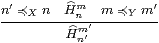
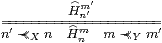
Lemma 16.5 The matrix is rounded, respecting ≺≺
on both sides, cf. Lemmas 11.7 & 15.2:
| ∃ m′. (m′≺≺Y m)∧ |
| nm′ ⇔ |
| nm ⇔ ∃ n′. |
| n′m∧ (n≺≺X n′). |
Proof
|
Lemma 16.6 Suppose n,m:N⊢ρ(n,m):Σ
satisfies the foregoing properties, i.e.
ρ(0,k)

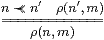
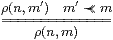
|
and define H:X−× Y by Hψ ≡ ∃ m n.Dmψ∧ρ(n,m)∧βn. Then ρ(n,m) ⇔ An(Hγm).
Proof Since ρ respects ≺≺ on the right,
|
Then, since ρ also respects ≺≺ on the left and An preserves the join, which is directed because ρ respects 0 and +,
|
Lemma 16.7 idnm ⇔ An(idβm) ⇔ (n≺≺ m) ⇔ Enm.
Proof The relationship with E follows from Lemma 14.5. The unit laws were given by Lemma 16.5, cf. the Karoubi completion, which splits idempotents in any category. ▫
Lemma 16.8 K· Hnk ⇔ ∃ m.Kmk∧Hnm.
Proof
|
although ⇐ is actually ⇔ as we have an ∨-basis. (We draw attention to this because [I] uses the natural ∧-basis on ℝ, and therefore the weaker result about composition.) ▫
Theorem 16.9 HS (Notation 5.13) is equivalent to the
category whose
The definition of HS in [A] was essentially taken from Hayo Thielecke’s work on “computational effects” [Thi97], which was in turn based on the Kleisli category for the monad. It was therefore motivated by more syntactic considerations than ours. From a semantic point of view, it would have been more natural to have split the idempotents. In the classical models, the category would then be the opposite of that of all continuous (but not necessarily distributive) lattices and Scott-continuous maps (cf. Example 2). In this result, we would drop the ≺≺+ and ≺≺⋆ rules from Definition 14.1 of an abstract basis.
In order to characterise first class maps, by Corollary 10.3 we have to consider preservation of the lattice connectives, cf. Lemmas 15.3ff. For this, the target object Y must have a lattice basis.
Lemma 16.10 H⊤=⊤ iff Hn1⇔(n≺≺ 1), and
H⊥=⊥ iff Hn0⇔(n≺≺ 0).
Proof If H⊤=⊤ then Hn1≡ An(Hγ1)≡ An(H⊤) ⇔ An⊤ ≡ Anβ1≡(n≺≺1) by Notation 16.1, Definition 6.6, and Notation 11.1.
Conversely, H⊤≡ Hγ1≡∃ n.Hn1∧βn ⇔ ∃ n.An⊤∧βn≡ ⊤ by Definition 6.6, Lemma 16.5 and Definition 6.2.
We may substitute ⊥ and 0 for ⊤ and 1 in the same argument. ▫
Similarly we are able on this occasion to handle ∧ and ∨ simultaneously (Remark 4.15).
Lemma 16.11 H(φ⊙ψ)=Hφ⊙ Hψ iff
Hns⊙ t ⇔
∃ m p.Hms∧Hpt∧ (n≺≺ m⊙ p),
both when ⊙ is ∧ or ⋆ and when it is ∨ or +.
Proof If H(φ⊙ψ)=Hφ⊙ Hψ then
|
Conversely, using distributivity,
|
Definition 16.12 An abstract matrix is a
binary relation Hnm such that
| 0m

|


|
Theorem 16.13 S is equivalent to the category whose
Jung and Sünderhauf characterised continuous functions between stably locally compact spaces in a similar way [JS96].
Remark 16.14 We shall speculate on the possible computational applications
of matrices for continuous functions in the next section,
but let’s say something here about the analogy
with linear algebra that we have used.
Really, this has been much more useful that we had any right to expect,
since neither S nor HS (the “first” and “second class” maps)
is a symmetric monoidal closed category.
However, by Theorem 9.11, stably locally compact objects and the A:X−× Y for which A preserves ⊤ and ∧ do define such a category. In fact, they provide a model of linear logic with involutive negation and an “of course” operator given by the Smyth powerdomain ℘♯ (Example 12.13):
Proposition 16.15
Let X be a stably locally compact space.
The HS-maps A:Γ−× X for which A:ΣX→ΣΓ
preserves ⊤ and ∧
correspond bijectively and naturally to S-maps Γ→℘♯X.
Proof Both correspond to terms Γ⊢ξ≡λ n.Aβn:ΣN that are rounded filters (∧-homomorphisms) for ≺≺X or ideals for ≻≻X. ▫
Since they also preserve directed joins, such A are known as preframe homomorphisms; for more on their relationship to the Smyth powerdomain, see [Vic88, 11.2.5] and [JKM01]. For a similar investigation of join-preserving maps and the Hoare or lower powerdomain ℘♭X in ASD, presumably we would first need to identify the “stably locally overt” objects to which the analogous construction may be applied.