


Definition 1.1
The traditional definition of local compactness was generalised
from Hausdorff to sober spaces in [HM81, p. 211]:
Whenever a point is contained in an
open subspace (x∈ V), there is a compact subspace K and an open
one U such that x∈ U⊂ K⊂ V.
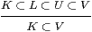
It is an easy exercise in the “finite open sub-cover” definition of compactness to replace the point x by another compact subspace:
Lemma 1.2
Let L⊂ V⊂ X be compact and open subspaces of a
locally compact space. Then there are
L ⊂ U ⊂ K ⊂ V ⊂ X
with U open and K compact. ▫
We call this result the interpolation property. Alternating inclusions of open and compact subspaces like this will be very common in this paper, and compact subspaces will be more important than points.
Notation 1.3 We write U≺≺ V and K≺≺ L
if there is such an interpolating compact or open subspace, respectively.
The second version, in which K⊃ L, follows the usage of
[HM81, JS96], cf. our Theorem 5.18.
Now consider what we might mean by a computably defined locally compact space.
Suppose that you have some computational representation of a space. It can only encode some of the points and open and compact subspaces, since in classical topology there are uncountably many of them in any interesting case. Hence your “space” cannot be literally sober, or have arbitrary unions of open subspaces. We understand the intended space to be the corresponding sober one, in which arbitrary unions of opens have also been adjoined. Those points, open and compact subspaces that have codes are called basic.
Example 1.4 A computable definition of ℝ as a locally compact
space might have
Notice that both open and closed intervals are used, although treatments of exact real arithmetic often just use one or the other, cf. Example 7.12. Also, by “rationals” we might actually mean all pairs p/q with integers p and q≠ 0, or the dyadic rationals p/2n, or continued fractions, or whatever our favourite countable dense set of reals may be. Unlike Dedekind cuts, this example readily generalises: for ℝ3 we use open and closed cuboids whose vertices have rational co-ordinates (or, better, a system based on close packing of spheres [CS88]).
In the Example, the intersection of two basic opens is again basic, but for technical reasons we shall also need to extend the families to include finite unions of open (respectively, compact) intervals or cuboids. It’s an exercise that’s a little too complicated to be called algebra, but easy programming, to test inclusion and compute the representations of such unions and intersections.
Definition 1.5
A computably based locally compact space consists of
a set of codes for basic “points”, “open” and “compact” subspaces,
together with an interpretation of these codes
in a locally compact sober space.
We require of the space that every open subspace be a union of basic ones.
We also want to be able to compute
Extensional equivalence of computable functions is not captured within the strength of the logic that we wish to study. So, for the “computations” above, we mean a particular program to be specified — at least up to provable equivalence, which means that we don’t have to nominate a programming language.
Definition 1.6 A computably continuous function
between such spaces is a continuous function f:X→ Y between the
topological spaces themselves, for which the binary relation
| f Km ⊂ Un |
(between the codes (n,m) for a compact subspace Km⊂ X and an open one Un⊂ Y) is recursively enumerable, cf. part (c) of the previous definition.
In particular, computably equivalent bases for the same space are those for which the identities in both directions are computably continuous functions. This means that the relations Kn⊂ Um and Km⊂ Un between n and m are recursively enumerable. For example, whilst there are several choices for the “rationals” and intervals in Example 1.4, all of the reasonable ones are computably equivalent.
Remark 1.7 It is out of place in the definition of
something computable to specify a topological space:
this was only included to guarantee topological consistency
of the computations of union, intersection, containment and interpolation.
This is also the reason why the codes for basic points
played no actual role in Definition 1.5 —
there needn’t be any of them.
Since we said that the spaces are sober,
continuous functions are determined entirely by their effect
on basic open and compact subspaces, as they are in locale theory.
Neither the (optional) basic points, nor the computable ones that
we recover in Section 15,
nor the uncountably many points of the classical theory,
are actually needed to specify continuous functions,
or prove topological properties such as compactness.
At the technical level, therefore, what we call a computably based locally compact “space” is really just a system of codes and programs acting on them, for which there exists a topological space in which these codes may be interpreted as compact and open subspaces. Likewise, a computably “continuous function” is just an equivalence class of programs, for which there exists a continuous function that agrees with the program in the way that we have said.
The particular way in which computations are set up is of course a matter for discussion: I still have to convince you of the merits of my way, in comparison to the many other ways that have been used to calculate in ℝn over the millennia, and of course any theoretical picture is subject to technical optimisation. However, these other ways share the same pattern, in that they have a technical definition that is (a) used for applied computation but (b) justified by the existence of an interpretation in some “pure” theory of (Euclidean) space. The pure theory is not the computation, at any rate if it is based on twentieth century topology. So the practical situation is illustrated by Example 1.4: we have a classical definition of a topological space, equipped with a basis that is defined in some conventional way, and which we want to use to obtain values in the space. So long as the above features of the basis are computable, the classical space guarantees the consistency conditions.
In Section 11 we shall formulate this consistency in terms of finitary conditions on the transformations of encodings themselves, eliminating the topological space, i.e. we prove necessity of the abstract conditions. Then in Section 14 we prove sufficiency, i.e. that any such encoding (such as the one for ℝ above) satisfying these consistency requirements does define a locally compact sober space, and this is unique up to homeomorphism.
This construction is done, not in traditional topology itself, which is not computable, but in a λ-calculus. Therefore, the construction imports the classical data into the computational world (Section 17). But again there is a distinction between the technical and philosophical meaning: whilst our theory (ASD) starts from (and is reducible back to) computational foundations, it adapts these to give a new account of the mathematical theory that is ultimately intended to be usable by pure mathematicians in place of the old one.
Remark 1.8 The operations ⋆ and + become
∩ and ∪ when we interpret them via the basic open
subspaces that they encode.
Amongst the abstract consistency requirements, therefore,
we would expect (0,1,+,⋆) to define a distributive lattice.
However, we have only asked for the ability to test inclusion of a compact subspace in an open one, not inclusion or equality of two open or two compact subspaces, nor of an open subspace in a compact one (the inclusion Un⊂ Kn is given, not tested). Even if these happen to be possible, it is computationally quite reasonable for different codes to denote the same subspace, but for this fact to be potentially undecidable.
On the other hand, as we want to stress the computable aspect of the names of basic subspaces, we shall often represent + and ⋆ as concatenations of lists. This clumsiness actually serves an expository purpose, keeping this “imposed” structure on codes separate in our minds from the “intrinsic” structure in the topology on X. (We shall regard this topology as another space.) If we used the notation and equations of a distributive lattice for the set N of codes, it would be all too easy to lapse into confusing it with the actual topology on the space. This would in fact make logical assumptions that amount to a solution of the Halting Problem (or worse).
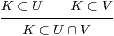
The topological information is actually contained, not in the quasi-lattice structure (0,1,+,⋆) on N, but in the inclusion relation between compact and open subspaces. This satisfies some easily verified properties:
 ▫
▫
|
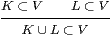
Finally, there is a property similar to Lemma 1.2 that concerns binary unions. Easy enough though this property may be to prove — when you see it — it is not something whose significance one would identify in advance. Various forms of it were originally studied by Peter Wilker [Wil70].
Lemma 1.10
Let K be a compact subspace covered by two open subspaces
of a locally compact sober space X, that is, K⊂ U∪ V.
Then there are compact subspaces L and M and open ones U′ and V′
such that
| K⊂ U′⋃ V′ U′⊂ L⊂ U and V′⊂ M⊂ V. |
Proof Classically, K∖ V is a closed subspace of a compact space, and is therefore compact too, whilst K∖ V⊂ U, so by the interpolation property (Lemma 1.2) we have
| K∖ V ⊂ U′ ⊂ L ⊂ U ⊂ X |
for some U′ open and L compact. Then K∖ U′ ⊂ K∖ (K∖ V) ⊂ V so
| K∖ U′ ⊂ V′ ⊂ M ⊂ V ⊂ X |
for some V′ open and M compact. Finally, K = (K∩ U′) ∪ (K∖ U′) ⊂ U′∪ V′. ▫
We didn’t mention the intersection of two compact subspaces in Definition 1.5, because there are spaces in which this need not be compact.
Definition 1.11 A locally compact sober space
is called stably locally compact if the whole space is compact
and the intersection of any two compact subspaces is again compact.