


Although our abstract re-axiomatisation is not quite complete (there are still two axioms to come, in the next section), we now have enough tools to fashion an account of the usual properties of compact subspaces based on the modal operator ▫ from Section 2. As in the traditional way in which compactness is taught, it seems to be easier to begin with compact subspaces of a Hausdorff space, and then consider compact spaces as a special case.
In Section 6 it was enough to refer to the open subsets such as δ and υ as propositional formulae. However, following Notation 2.14, we shall now need to use a “general” or “arbitrary” open subspace φ in a test of the form ▫φ to examine compact subspaces. This is why we needed to introduce λ-abstraction in the previous section.
In Section 2 we wrote ▫U for the property that a compact subspace K is contained in an open one U. Now we shall allow ▫ to stand for an expression that may quite naturally contain variable parameters. This will enable us to treat abstract compact subspaces as intermediate expressions in the course of calculations that have real-valued inputs and outputs, such as the solution of polynomial equations. Working with higher-type expressions is much simpler, both notationally and conceptually, than trying to understand what it means for a compact set K to depend continuously on parameters.
Definition 8.1
An abstract compact subspace of a Hausdorff space H
is defined by its necessity modal operator.
This is an expression ▫, possibly containing parameters,
that yields a proposition (term of type Σ)
when applied to an open subset (term of type ΣH),
so by Axiom 7.4 its own type is ΣΣH.
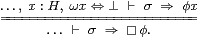
As in Notation 2.14, ▫ must satisfy, for any predicate-expression φ:ΣH,
| ▫φ ⇔ ⊤ ⊣⊢ φ∨ω = ⊤ where ω x ≡ ▫(λ y.x≠H y). |
If we want to name the subspace, we write [K]φ instead of ▫φ. The intended meaning is that the compact subspace K represented by ▫ is contained in (or covered by) the open subspace classified by φ.
In English, the formula ω x≡▫(λ y.x≠ y) reads: “x belongs to the complementary open subspace (called W in Section 2) iff, necessarily for any y in the subspace, x is separated from y”. The symbol ▫ says “necessarily, in the compact subspace”, whilst ≠ denotes separation in a Hausdorff space (Definition 4.8).
Proposition 8.2
For a:H, σ:Σ, φ,ψ:ΣH and
θ:ΣH1× H2, ▫ operators obey
Proof [a] For any φ, by hypothesis ▫φ⇔⊤⊣⊢φ∨ω⇔⊤⊣⊢▫′φ⇔⊤, so ▫φ⇔▫′φ by Axiom 5.6. [b] ⊤∨ω=⊤, whilst
| φ∨ω=ψ∨ω=⊤ ⊣⊢ (φ∨ω)∧(ψ∨ω)=⊤ ⊣⊢ (φ∧ψ)∨ω=⊤ |
by distributivity. [c] Putting Fσ ≡ ▫(λ x.σ∨φ x) in Proposition 5.8, we have
| F⊤ ≡ ▫(λ x.⊤∨φ x) ⇔ ▫(λ x.⊤) ≡ ▫⊤ ⇔ ⊤ |
and
| F⊥ ≡ ▫(λ x.⊥∨φ x) ⇔ ▫(λ x.φ x) ≡ ▫φ, |
so ▫(λ x.σ∨φ x) ≡ Fσ ⇔ F⊥∨σ∧ F⊤ ⇔ ▫φ∨σ∧⊤ ⇔ ▫φ∨σ.
[d] Relative instantiation is the forward direction of the defining rule (using Axiom 5.6 and λ-application) and [e] the substitution property is simply that for λ-application (Axiom 7.7). [f] Using the Definition and Axiom 5.6, (equality with ⊤ of) the left hand side of the commutative law is equivalent to
|
which is symmetric, so agrees with the other side. ▫
Definition 8.3 If ▫ is covered by φ
then φ is called a neighbourhood of ▫.
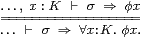
A point a:H (by which we mean an expression that may contain parameters)
belongs to all such neighbourhoods φ if
| ▫φ=⇒ φ a, or ▫ ⊑ λφ.φ a:ΣΣH |
using Notation 7.8. This agrees with
| a∈ K, where K ≡ {x:H ∣ ▫⊑λφ.φ x} |
is defined using Notation 7.15, so we say that a is a member of ▫.
Warning 8.4 Without the Hausdorffness assumption
(and interpreting it in traditional topology),
this definition need not recover membership of a given compact subspace,
but may give a larger one,
called the saturation [HM81].
Example 8.5
Any point of a Hausdorff space defines a compact subspace K≡{a},
with [K]φ≡φ a and ω x≡(x≠ a),
by Lemma 5.9.
Then [K] preserves meets and joins, cf. Proposition 2.15(d). ▫
Definition 8.6 We say that a compact subspace K
is occupied if [K]⊥⇔⊥,
whereas [K]⊥⇔⊤ iff K≅∅,
cf. Proposition 3.
Any compact subspace that has a definable point is occupied, but not conversely. For example, we shall see that any function I→ℝ attains its bounds (or any particular intermediate value) on an occupied subspace (Corollaries 12.13 and 13.11), but not necessarily at any point of it (Example 16.15). To appreciate why the word was chosen, imagine going into a hotel room to find someone else’s luggage already there, but not the actual person. The more familiar notion of inhabitedness says that a point exists, so it will be related to ∃ and ◊ for overt subspaces in Definition 11.5. When we return to the intermediate value theorem in Section 14, we shall see that the fact that occupied subspaces need not have points exactly explains the difference between the classical and constructive views of the result (Corollary 14.16).
Proposition 8.7
Any compact subspace of a Hausdorff space is closed.
Proof As we explained in Remark 7.16, we have to show that the two subspaces that are defined from the data for compactness and closedness are isomorphic. We do this by proving that their defining statements,
| ▫φ=⇒φ x and ω x ⇔ ⊥, |
are equivalent. If the first holds then, putting φ≡λ y.(x≠ y) in the first form of Definition 8.3,
| ω x ≡ ▫(λ y.x≠ y) =⇒ (λ y.x≠ y)x ≡ (x≠ x) ≡ ⊥. |
Conversely, if ω x⇔⊥ then ▫φ⇒φ x for any φ:ΣH, by Proposition 4. ▫
Examples 8.8
The empty subspace is compact, as are binary unions and
intersections of compact subspaces of a Hausdorff space.
|
According to Definition 7.17, the intersection of a pair of subspaces is given by the conjunction (&) of their defining statements, but
| (ω1 x⇔⊥) & (ω2 x⇔⊥) ⊣⊢ (ω1 x∨ω2 x)⇔⊥ |
is the definition of ∨, so the intersection of the two closed subspaces is closed. The same is true of the compact ones because of the equivalence of closed and compact subspaces of either K1 or K2 in Theorem 8.15 below. ▫
Although we have not defined unions of general subspaces, next result shows that what we have called K1∪ K2 is the direct image of the coproduct (disjoint union) K1+K2.
Theorem 8.9
Let f:X→ Y be a function (Definition 5.3)
between Hausdorff spaces, and let K be a compact subspace of X.
Then
| [f K]ψ ≡ [K](f*ψ) ≡ [K](λ x.ψ(f x)) |
defines a compact subspace f K⊂ Y, called the direct image of K. If a:X is a member of K⊂ X then f a:Y is a member of f K⊂ Y, and f K is occupied iff K is.
Conversely, f:K↠ f K is a proper surjection in the sense that the inverse image f−1(y)∩ K⊂ X of each y∈ f K⊂ Y is compact and occupied.
Proof Since X and Y are Hausdorff, we may define
| ξ x ≡ [K](λ x′.x≠ x′) and ω y ≡ [f K](λ y′.y≠ y′) ≡ [K](λ x. y≠ f x). |
By hypothesis, [K]φ⇔⊤ iff φ∨ξ=⊤:ΣX, and we have to show that [f K]ψ⇔⊤ iff ψ∨ω=⊤:ΣY.
|
If ψ∨ω=⊤:ΣY then (ψ· f∨ξ)=⊤:ΣX, so [K](ψ· f) ≡[f K]ψ⇔⊤, by the first part. Conversely, from the second, if [f K]ψ⇔⊤ then (ψ∨ω)=⊤:ΣY.
If a∈ K, so [K]φ⇒φ a, then [f K]ψ ≡ [K](ψ· f) =⇒ (ψ· f) a ≡ ψ(f a), so f a∈ f K. Also, [f K]⊥ ≡ [K](⊥· f) ≡ [K]⊥ ⇔ ⊥.
Since Y is Hausdorff, {y} and f−1(y) are closed, by Lemma 7.20. the intersection f−1(y)∩ K exists, and is closed and compact by Example 8.8, with
| [f−1(y)⋂ K]φ ⇔ [K](λ x.y≠Y f x∨φ x), |
so
| [f−1(y)⋂ K]⊥ ⇔ [K](λ x.y≠Y f x) ≡ ω y. |
Hence f−1(y)∩ K is occupied iff y∈ f K⊂ Y. ▫
We now turn from subspaces to spaces.
Definition 8.10
A space K is compact if it has
a universal quantifier, written ∀K,
such that, for x:K and φ:ΣK,
| ∀K⊤⇔⊤ and ∀Kφ=⇒φ x, |
the latter being called the absolute instantiation rule. In other words, K is a compact subspace of itself with ω≡⊥, and any expression of type K is a member of ▫ in the sense of Definition 8.3. (This simple definition is sufficient because of Axiom 5.6.)
We look at the logical meaning of this before the topological one.
Notation 8.11 We shall write ∀ x:K.φ x for ∀Kφ
when K is a compact space, and by extension also
when it is a compact subspace, i.e. for [K]φ.
This simply means that we replace the notation
| ▫(λ x:K.⎯⎯) by ∀ x:K.⎯⎯. |
This use of logical notation is justified by Proposition 8.2 and the following rules of inference.
Warning 8.12 The quantifier ∀ must be understood strictly
according to the rules in this section, cf. Remark 5.1.
It does not mean “for every definable point”.
There is an occupied compact subspace that has no points at all
(Example 16.15) and
even the real interval I may satisfy ⊢φ a
for every term ⊢ a:I but not ∀ x:I.φ x
Section I 15.
Theorem 8.13
In a compact space, ∀K satisfies the two-way rule on the left:
|
where σ:Σ must not involve the variable x:K. This is the dual of Axiom 5.10 for ∃. Similarly, in a Hausdorff space H, the modal operator ▫ and co-classifier ω for a compact subspace satisfy the rule on the right.
Proof By Axiom 5.6 and Notation 7.8, the rule on the right above is
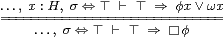 or
or
|
which is Definition 8.1. The other rule is the special case where ω x ≡ ⊥. ▫
Lemma 8.14 In a compact Hausdorff space,
φ x ⇔ ∀ y.(x≠ y)∨φ y.
Proof This is the dual of Lemma 5.14 for overt discrete spaces.
|
From this we deduce the familiar topological result.
Theorem 8.15
The closed and compact spaces of a compact Hausdorff space agree, where
| ω x ≡ ▫(λ y.x≠ y) and ▫φ ≡ ∀K(φ∨ω) ≡ ∀ x:K.φ x∨ω x |
translate between ω and ▫.
Proof When the ambient space is compact, the right hand side of the rule in Definition 8.1 is equivalent to ∀K(φ∨ω)⇔⊤, so these two equations re-state that Definition. Proposition 8.7 showed that the two notions of membership agree.
The translation ω↦▫↦ω′ is the identity by Lemma 8.14:
| ω′ x ≡ ▫(λ y.x≠ y) ≡ ∀K (λ y. x≠ y∨ ω y) ⇔ ω x. |
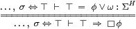
So too is that ▫↦ω↦▫′, by Axiom 5.6 and because
| ▫′φ⇔⊤ ⊣⊢ ∀K(φ∨ω)⇔⊤ ⊣⊢ φ∨ω=⊤ ⊣⊢ ▫φ⇔⊤. ▫ |
Being compact as a subspace was defined in terms of the topology of the ambient space. Before we can say that the subspace is compact as a space in its own right, we have to define its own topology. We can do this, using Axiom 7.10, if the subspace is also either closed or open. Recall, however, that we may only form the type C from an operator ▫ if it has no parameters. This is why we prefer to work with this operator instead of the space, and subsequent results will not depend on forming it.
Theorem 8.16
Any compact subspace of a Hausdorff space is itself
a compact space.
Proof From ▫:ΣΣH define ω x≡▫(λ y.x≠ y) and C≡{x:H ∣ ω x⇔⊤} using Axiom 7.9. Then, by Axiom 7.10, the topology of C has
| I:ΣC≅{φ:ΣX ∣ ω⊑φ}↣ΣX, |
and we use this Σ-splitting I to define ∀Cψ≡▫(Iψ). This satisfies absolute instantiation for x:C and ψ:ΣC,
| ∀Cψ ≡ ▫(Iψ) ≡ ▫ψ =⇒ ω x∨ψ x ≡ ψ x |
because ω x⇔⊥ and ω⊑ψ=Iψ, whilst ∀C⊤≡▫(I⊤C)≡▫⊤X⇔⊤. ▫
Remark 8.17
Returning to logic, the significance of the deduction rule for subspaces
(on the right in Theorem 8.13)
is that we may treat ▫ as a bounded universal quantifier.
For example, in Section 10 we shall consider, for d,u:ℝ and φ:Σℝ,
| ▫φ ≡ [d,u]φ ≡ ∀ x:(d≤ x≤ u).φ x. |
That is, we can reason about it as if the subspace
| K ≡ {x:H ∣ ¬ω x} = {x:H ∣ ▫⊑λφ.φ x} ⊂ H |
were actually a space in its own right (even when ω and ▫ depend on parameters).
Remark 8.18
This account of compact subspaces has relied on the Hausdorffness assumption,
which ought to be enough, given that we intend to study ℝ and ℝn.
However, when we introduce (closed) overt subspaces in Section 11,
we would like to do so in the form of the lattice dual
of the theory of (open) compact subspaces (cf. Axiom 5.6),
whereas ℝ does not enjoy the dual property to Hausdorffness,
which is discreteness.
A small detour from the topology of ℝn is therefore appropriate.
There are ample supplies of open compact subspaces in
Definition 8.19
A compact open subspace of a (not necessarily Hausdorff) space X
is defined by a pair (▫,α),
where ▫:ΣΣX and α:ΣX satisfy
| ▫φ ⇔ ⊤ ⊣⊢ α ⊑ φ |
for any φ:ΣX. Equivalently (by Axiom 5.6), ▫φ∧α x=⇒φ x and ▫α ⇔ ⊤.
| x,y:X, α1 x⇔α1 y⇔⊤ ⊢ φ x y⇔⊤; |
|