


When we have described our new λ-calculus for general topology, we shall apply it to the intermediate value theorem, which solves equations that involve continuous functions ℝ→ℝ.
The usual constructive form of this result puts an additional condition on the continuous function, where the classical one has greater generality. Also, the constructive argument is based on an interval-halving method that apparently gives just one extra bit of the solution for each iteration, whereas the well known Newton algorithm doubles the precision (number of bits) each time.
Whilst it is widely appreciated that constructivism emphasises similar issues to those that arise in computational practice [Dav05], classical analysts sometimes feel that their constructive colleagues want to rob them of their theorems, without replacing them with algorithms that are any better than those that numerical analysts already know.
When we look more closely into these complaints, we find that the two sides are talking at cross-purposes and even the traditionalists are conflating two different theorems of their own. Some mathematicians consider the “generality” of classical results to be more important than their applications. On the other hand, anyone who is genuinely interested in solving an equation, i.e. in finding a number, will probably already have some algorithm (such as Newton’s) in mind, and will be willing to accept the pre-conditions that this imposes. We find, on examination, that these imply the extra property that constructivists require, which is in fact very mild: it is satisfied by any example in which you might reasonably expect to be able to compute a zero. Topologically, these conditions are weaker forms of openness, whilst the “general” theorem is about continuous functions.
Turning to the classical Newton algorithm, it is not always as good as it claims: on the large scale it can run away from a nearby zero and sometimes behaves chaotically. In fact, it only exhibits its rapid convergence after we have first separated the zeroes, which we must do by some discrete method such as interval-division. Ramon Moore’s interval Newton method [Moo66, Chapter 7], which exploits Lipschitz conditions instead of differentiability (cf. Definition 10.9), behaves at small scales like its traditional form, but at larger ones like interval halving, so it finds the initial approximation to the zero in a systematic way. Andrej Bauer has begun to demonstrate that computation may indeed be performed efficiently in the ASD calculus using these methods [Bau08].
Constructive mathematics is about proving theorems just as much as classical analysis is. What we gain from looking at the intermediate value theorem constructively is a more subtle understanding of the space of solutions in the singular and non-singular situations. In this paper, this will take the form of a new topological property of the space Sf of “stable” zeroes, which are essentially those that can be found computationally. Nevertheless, the space Zf of all zeroes (stable or otherwise) still plays an equally important role: we shall study the two together, in a way that is an example of the open–closed duality in topology.
Let us begin, therefore, with the form in which the (classical) intermediate value theorem is taught to mathematics undergraduates:
Theorem 1.1
Let f:I≡[0,1]→ℝ be a continuous function
with f(0)≤ 0≤ f(1).
Then there is some x∈I for which f(x)=0.
Proof There are two well known proofs of this.
| xn≡½(dn+un), and put dn+1, un+1 ≡ | ⎧ ⎨ ⎩ |
|
These methods are not suitable as they stand for numerical solution of equations:
Example 1.2
Consider this parametric function, which hovers around 0:
| for −1≤ s≤ +1 and 0≤ x≤ 3, let fs(x) ≡ min(x−1, max (s, x−2)). |
The graph of fs(x) against x for s≈ 0 is shown on the left. The diagram on the right shows how fs(x) depends qualitatively on s and x, where the two regions are open, and the thick lines denote fs x=0. In particular, f(1)=0 iff s≥ 0, f(2)=0 iff s≤ 0 and f(3/2)=0 iff s=0.
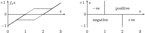
Neither the classical theorem nor any numerical algorithm has much to say about analysis in this example. However, if any of them does yield a zero of fs, as a side-effect it will decide a question of logic, namely how s stands in relation to 0.
Remark 1.3
As L.E.J. Brouwer observed in his revolutionary work in 1907
[Bro75, Hey56],
for an arbitrary numerical expression s,
we may not know whether s< 0, s=0 or s> 0.
There are many different ways in which such indeterminate values may arise,
depending on whether your reasons for using analysis come from
experimental science, engineering, numerical computation or logic.
So s may be
| gn ≡ | ⎧ ⎨ ⎩ |
|
We see that the issue is one of logic rather than geometry
and the definitive answer only came in the 1930s.
Whether Bolzano, Cauchy or the other 19th century analysts and geometers
would have intended the intermediate value theorem to apply to
Brouwer’s example is a question that needs extremely careful
historical investigation.
Other errors were made because
the notion of uniformity was lacking (Remark 10.11),
for example,
so the fair conclusion is that those who believed the general result
were relying on decidable equality of real numbers,
and as such were mistaken in this too.
Since the Example is a monster from logic and not analysis, we bar it [Lak63]. It is also sometimes more convenient to suppose that the function is defined on the whole line.
Definition 1.4
We say that f:ℝ→ℝ doesn’t hover if,
| for any e< t, ∃ x.(e< x< t) ∧ (f x≠ 0), |
so the open non-zero set Wf≡{x ∣ f x≠ 0} is dense. A similar property, that f is “locally non-constant”, is used in other constructive accounts such as [BR87].
Example 1.5 Any non-zero polynomial of degree n doesn’t hover, x being
one of any given n+1 distinct points in the interval (d,u). ▫
Remark 1.6 For Newton’s algorithm to be applicable to solving the
equation f(x)=0, we must assume that the derivative f′ exists,
and preferably that it is continuous.
Also, since we intend to divide by f′(x), this should be non-zero,
although it is enough that f′ doesn’t hover.
So let d< x′< u with f′(x′)≠ 0.
Then, by manipulating the inequalities in the ε–δ
definition of f′(x′), cf. Definition 10.9,
there must be some d< x< u with f(x)≠ 0.
This argument may be adapted to exploit any higher derivative
that is non-zero instead. ▫
So this condition is very mild when taken in the context of its practical applications. Using it, here is the usual (exact) constructive intermediate value theorem (there is also an “approximate” one, cf. Proposition 13.4).
Theorem 1.7
Suppose that f:ℝ→ℝ is continuous,
has f(0)< 0< f(1) and doesn’t hover.
Then it has a zero.
Proof In the interval-halving algorithm (Theorem 2), we may have f(xn)=0. This can be avoided by relaxing the choice of xn to the x provided by Definition 1.4, to which we supply, say, e≡⅓(2dn+un) and t≡⅓(dn+2un). Then we only have to test whether f(xn)< 0 or > 0, which is allowed, both constructively and numerically [TvD88, Theorem 6.1.5]. ▫
This proof is better computationally than the previous one, in that it doesn’t involve a test for equality. But it introduces a new problem: the meaning of ∃, to which we shall return many times. Here we characterise the solutions that this algorithm actually finds.
Definition 1.8
We call x∈ℝ a stable zero of f if,
for any d< x< u,
| ∃ e t.(d< e< t< u) ∧ (f e< 0< f t ∨ f e> 0> f t), |
leaving you to check that a stable zero of a continuous function really is a zero. Stable zeroes are elsewhere called transversal.
On the other hand, even in such a nice situation as solving a polynomial equation, not all zeroes need be stable — in particular, double ones (where the graph of f touches the axis without crossing it) are unstable. As Example 1.2 shows, if f hovers, there need not be any stable zeroes.
Example 1.9
Consider fs x ≡ s x2−s x+1 for s> 0 and 0≤ x≤ 1,
so fs 0=fs 1=1.
There are two stable zeroes when s> 4,
a single unstable one at ½ when s≡ 4,
but no zeroes at all when s< 4 . ▫
This discussion may perhaps suggest that unstable zeroes are a bad thing. However, the computational results are only one side of what we have to say in this paper: our treatment of topology will consider both stable and arbitrary (i.e. either stable or unstable) zeroes. In fact, it is also possible to compute unstable zeroes, if they are isolated and we know that they’re there, but this is a distraction from our story.
We conclude this section with a couple of remarks concerning the choice of name and formulation of stable zeroes.
Remark 1.10
Earlier drafts of this paper required e< x< t
in Definition 1.8.
Suppose we have e< t< x, where f e and f t have opposite signs,
and f doesn’t hover in the interval (x,u).
Then f y< 0 or f y> 0 for some x< y< u,
so we may replace either e or t with y
to obtain the stronger property.
Similarly, if there are stable zeroes arbitrarily close on both
sides of a point then it is a stable zero in the stronger sense.
Example 1.11 The hovering function
f(x)≡sin(π/ x) if x> 0 and 0 if x≤ 0
has stable zeroes in the stronger sense at 1/n
but only in the weaker one at 0. ▫
Remark 1.12 (Andrej Bauer)
We call such zeroes stable because, classically,
x is a stable zero iff
every nearby function (in the sup or ℓ∞ norm) has a nearby zero:
| ∀δ> 0. ∃ε> 0. ∀ g. (|f−g|≤ε=⇒ ∃ y. g y=0 ∧ |y−x|<δ). |
However, the ∀δ, ∀ g and = in this formula mean that it is not a well formed predicate in the calculus that we shall introduce in this paper, although the ∀ g may be allowed in a later version.