


In the previous section we defined the translation X of each type X simply by erasing comprehensions. Although the inclusion map iX:X↣ X was more complicated, we shall now see that the corresponding translation a of terms is equally simple: erase the connectives i and admit, but replace (the in any case unnatural) I with E .
Notation 10.1
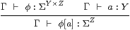
By structural recursion on terms, we define the translation
|
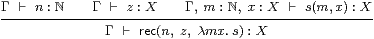
| ≡ rec ( |
| , |
| , λ m |
| . |
| ) |
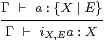
For the variable x:X, the symbol x (either as a term or as a λ-binding) is not a translation as such, but a new variable of type X . We shall also define
| ≡ force |
| . |
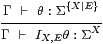
Notice that focus is not translated into focus, and we shall not allow terms to involve it in the main part of the discussion. The problem is that the translation Γ⊢ P :Σ2 X does not respect the equation that says that P is prime and so justifies use of the focus operator. However, from Lemma 8.13 and Proposition A 8.10, focus is only needed on the outside of a term, and then only for type ℕ, so we shall deal with it separately at the end of the section.
Notation 10.2 For any context Γ, define Γ
by replacing each typed variable x:X in Γ
by x : X .
Similarly, let iΓ:Γ↣Γ
be the list of [iX(x)/ x ]:X↣ X .
We write iX* and iΓ* for the substitutions
that relate terms involving these free variables,
whereas ΣiX relates the corresponding λ-abstractions,
cf. Lemma 10.7 below.
Hence
| i[ ]* |
| ≡ |
| and i[Γ, x:X]* |
| ≡ [iX(x)/ |
| ]* iΓ* |
| . |
Most of this section is devoted to proving
Theorem 10.3
For any term Γ⊢ a:X in the comprehension calculus
without focus,
Γ⊢ a : X
is well formed in the original calculus, whilst
| Γ ⊢ a = admitX(iΓ* |
| ):X and Γ ⊢ iX a = iΓ* |
| : |
|
are provable in the comprehension calculus, i.e. the square
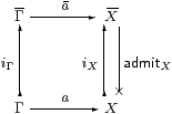
commutes. The two forms are equivalent by the {}β and {}η rules, Lemmas 9.9 and 9.10.
In particular, if Γ and X don’t involve comprehension then Γ⊢ a= a :X.
The proof is by structural induction on the term Γ⊢ a:X, and therefore has a case for each connective: λ, i, admit, I, etc. Each of these cases is a lemma below, whereas the lemmas in the previous section were self-contained. To avoid repetitious language, the enunciation of each lemma is simply the introduction or elimination rule that defines the connective; by this we mean to assert that “if the premises (sub-terms) obey the equation a=admitX(iΓ* a ) then so does the conclusion”.
Since the transformation is also applied to nuclei (Lemma 10.10), the proof is actually on the history of formation of a, rather than simply on the expression without type annotations.
Variables, constants and algebraic operations
Lemma 10.4 For x:X⊢ x:X, we have admitX(iX* x ) = x.
Proof iX* x = [iX x/ x ]* x = iX x, and admitX(iX x)=x by Lemma 9.10 ({}η for X). ▫
There is nothing to prove for the constants ⊤, ⊥ and 0, and almost nothing for succ, so we just consider ∧ as (an example of) an algebraic operation.
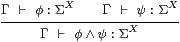
Lemma 10.5
|
Recall from the statement of Theorem 10.3 that, by displaying this rule, we mean to claim that if φ and ψ satisfy a certain equation then so does φ∧ψ.
Proof The general plan is to expand the term in the conclusion of the rule (here φ∧ψ), using the induction hypothesis for the sub-terms (here φ and ψ) and the formulae for admit (Notation 9.2) and iΓ* (Notation 10.2), then apply the extended “rules” from the previous section, followed by the same procedure in reverse to obtain the translation of the term in question.
|
Lemma 10.6
|
Proof
|
The lambda calculus
The difference between ΣiY and iY* is that
ΣiY acts on the exponent of the type by λ-reduction,
whilst iY* acts on the context by substitution.
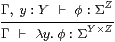
Lemma 10.7
If Γ, y : Y ⊢θ:Σ Z then
Γ⊢ΣiY× iZλ y .θ =
λ y.ΣiZiY*θ:ΣY× Z.
Proof
|
Lemma 10.8
|
Proof We use Lemma 10.7 with Γ, y : Y ⊢θ ≡ iΓ* φ :Σ Z .
|
|
Proof
|
Subtypes
Here is where we use the main induction hypothesis in Theorem 10.3
for the nucleus E that defines the subtype {X ∣ E}.
The prohibition on focus is not a problem:
it can be eliminated, as the type of E is ΣX
(Proposition A 8.10).
Lemma 10.10 ΣiX· E =E·ΣiX
and E{X ∣ E}=IX· E·ΣiX= E .
Proof The induction hypothesis for Eφ and φ yields
| Eφ = admitΣX( |
|
| ) = ΣiX( |
|
| ) and φ = admitΣX |
| = ΣiX |
| , |
so E(ΣiX φ ) = ΣiX( E φ ), which is the first equation. The induction hypothesis also says that EX= EX , since the type of EX doesn’t involve comprehension. Then
| E{X ∣ E} = IX· E·ΣiX = IX·ΣiX· |
| = EX· |
| = |
| = E |
by Notation 10.2 and Lemmas 9.4, 10.9 and 9.8. ▫
Lemma 10.11

|
Proof
|
Lemma 10.12
|
Proof
|
Lemma 10.13
|
Proof
|
Recursion
Lemma 10.14
|
[This proof requires equational hypotheses (Remark E 2.7).]
Proof Let Γ⊢ z′=iΓ* z : X and Γ, m:ℕ, x : X ⊢ s′(m, x )=iΓ* s (m, x ): X .
So the induction hypotheses say that Γ⊢ n=iΓ* n :ℕ, Γ⊢ z=admitX z′:X and
| Γ, m:ℕ, x:X ⊢ s(m,x)=admitX s′(m,iX x):X. |
We use Lemma 8.14, or rather its analogue with the extended rules of Section 9 in place of the {}β- and η-rules; the symbols x , z′ and s′ here correspond to y, z and s there.
|
Sobriety
We have now completed the proof of Theorem 10.3,
that, for any term Γ⊢ a:X in the comprehension calculus
without focus,
| Γ ⊢ a=admitX(iΓ* |
| ):X and Γ ⊢ iX a = iΓ* |
| : |
| . |
There are two ways of handling a term focusP:ℕ.
Remark 10.15 Lemma 8.11 says that
ℕ≅{Σ2ℕ ∣ Eℕ},
where Eℕ characterises primes.
This makes use of admit instead of focus.
More generally, {ℕ ∣ E}≅{Σ2ℕ ∣ E′},
where E′ encodes the composite inclusion.
Another way of saying this is that, in Notation 9.2,
we define the base case ℕ
as Σ2ℕ instead of ℕ.
This way we only ever deal with subspaces of injectives
(cf. Corollary 5.3), and never need to use focus.
Remark 10.16 Alternatively,
if Γ⊢ P:Σ2 X is a prime not involving focus,
|
Lemma A 8.4 actually said
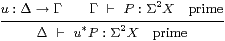
|
| Δ ⊢ u*(focusP) = focus(u*P) :X |
and we’re trying to use its converse, which is not valid. Although Γ⊢ iΓ* P :Σ2 X is prime, Γ⊢ P :Σ2 X need not be. This is why we write force instead of focus here.
Semantically, Γ↣Γ is a subspace, on which the relevant equation holds, but it need not hold on the ambient space Γ. That such a situation arises is more obvious for descriptions (Remark A 9.13): any predicate Γ⊢φ:Σℕ becomes a description when restricted to the locally closed subspace Γ↣Γ defined by
| (∃ n.φ[n]) ⇔ ⊤ and (∃ n m.φ[n]∧φ[m]∧ n≠ m) ⇔ ⊥. |
In the terms of this paper, the equation in Definition 4.5 defining a (prime or) homomorphism on a subspace {Y1 ∣ E1} involves E1, and does not imply the form without it.
Nevertheless, it is a legitimate alternative way of treating focusP to translate it into force P . For, if Γ⊢ψ:ΣX then
| ψ[focusP] ⇔ Pψ ⇔ (admitΣ2 XiΓ* |
| )(admitΣX iΓ* |
| ) ⇔ iΓ* |
| ⇔ iΓ* |
| [force |
| ] |
using the unrestricted β-rule for force.
As we know from Section A 8 and 11, and the work on computational effects cited there, we may obtain different terms Γ⊢ a : X by applying or reversing the β- and η-rules of the λ-calculus with force. So, for such a calculus to be defined consistently, an order of evaluation must be specified.
However, these computational terms with possibly different denotations on Γ become equal when we apply iΓ* to restrict them to the required context Γ. In other words, as we know very well from experience, there are different programs Γ⊢ a : X , possibly involving computational effects, to compute the same denotational value Γ⊢ a:X.
Categorical equivalence
Theorem 10.17 Let S and D be the categories generated by the restricted
λ-calculus (possibly with the extra structure)
and the comprehension calculus.
Then there is an equivalence of categories S≃D
whose effect on types is
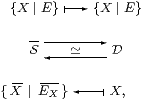
where the notation {X ∣ E} in S is the categorical one in Section 4, whilst in D it is understood as the comprehension calculus in Section 8.
Proof The previous section defined the transformation D→S on types, and showed that the composite D→S→D is isomorphic to the identity: Proposition 9.11 provided mutually inverse terms in the comprehension calculus that relate any type X to { X ∣ EX}. The other composite is the identity on types, so we just have to show that S→D is full and faithful.
Let X1 and X2 be types that are defined without comprehension, and E1 and E2 nuclei on them. We shall show that there is a bijection between the S-morphisms
| :{X1 ∣ E1}—→{X2 ∣ E2} |
defined in Section 4 and the terms
| x:{X1 ∣ E1} ⊢ focusP:{X2 ∣ E2} |
that we have just expressed in normal form. Of course {X1 ∣ E1} =X1, and we write i1=iX1, etc.
In each of the categories, these morphisms correspond bijectively to homomorphisms
| Σ{X2 ∣ E2}—→Σ{X1 ∣ E1}, |
but first we consider ordinary maps, without the homomorphism requirement.
By Proposition 6.2 for S, Σ{X ∣ E}≅{ΣX ∣ ΣE}, which is simply a retract of the power type ΣX in S (the restricted λ-calculus), so a S-morphism J:Σ{X2 ∣ E2}→Σ{X1 ∣ E1} is a S-morphism J:ΣX2→ΣX1 such that E2;J=J=J;E1.

The corresponding power type in D is also a retract, and Theorem 10.3 characterised its morphisms H in the same fashion. Hence HS≃HD.
Now, homomorphisms are characterised equationally amongst all maps, and we have already shown that the functor is full and faithful for them, i.e. that maps and their equations agree, so the homomorphisms also agree.
In S, the equation that defines homomorphisms is more clearly understood by means of Lemma 6.6, i.e. with reference to the subtypes {Xi ∣ Ei}, rather than using Definition 4.5, which transfers the condition to the ambient types Xi. We have seen the same phenomenon in D, where the translation P of a prime P relative to the sub-types need not be prime with respect to the translated types.
That deals with single-type contexts, but that is enough as products may be encoded as comprehension types in each category. ▫
Therefore our first construction, adjoining formal Σ-split equalisers to the category in Sections 4–6, is equivalent to the third, the extension of the λ-calculus in Sections 8–10.