


In ASD, as in classical topology and locale theory, I and ℝ are connected in senses that test not just pairs of open or clopen subspaces, as we did in Section 13, but sets of them. We make this generalisation in two steps, one finitary and the other infinitary, of which the second uses Heine–Borel compactness and so fails in Bishop’s theory. We deduce that the decomposition of any open set into intervals (Theorem 13.15) is unique (this is called local connectedness) and that any occupied compact interval [δ,υ] is compact connected. Finally, we relate the notions of connectedness from constructive analysis to those that have been used in category theory.
Remark 15.1
The principal arguments in this section are combinatorial,
manipulating lists of rational numbers.
These rely on the theory of compact overt subspaces of overt discrete spaces,
of which we gave a sketch in Remark 12.16;
the details are in
Section C 10
and [E].
In the following lemma, we build up a permutation p of m≡{i:ℕ ∣ i< m} as a composite of swaps. This uses either group theory or programming, but both in a very simple way. Unfortunately, the simplest proof of this kind becomes extremely complicated if we dwell on the minutiae of formal logical calculi. Besides the issues in Remark 12.16, it is important to understand how the formalities relate to the usual idioms of mathematics: this is explained in [Tay99, §§1.6 & 6.5].
Note in particular that the quantifier ∃ p in the following lemma, which ranges over the group of permutations of ℕ that have finite support, is justified because such permutations may be encoded as integers, so this group is an overt discrete space.
The quantification over lists in Theorem 15.10 is even more delicate than this. It is essential that we work over the overt discrete space ℚ. There, any compact overt subspace is (also discrete and so) Kuratowski-finite, which means that it may be expressed as a finite list, possibly with repetitions. As we saw in Section 12, compact overt subspaces of ℝ are entirely different beasts.
Lemma 15.2
Let θ0,…,θm−1 be open subsets of a space X that
are each inhabited in, and together cover, an overt connected subspace
S⊂ X defined by ◊, so
| …, i:ℕ ⊢ θi:ΣX, ◊θi⇔⊤ and … ⊢ m:ℕ, (∃ i< m.θi)=⊤S. |
Then the overlaps of the θi define a connected graph, in the sense that there is some permutation p:m≅m for which
| ∀ i:(1≤ i< m). ∃ j.(0≤ j< i) ∧ ◊(θp(i)∧θp(j)). |
Proof In the subsequent infinitary argument we shall need the number m here to be a parameter, so we extend the definition of θi to all i:ℕ by putting θi≡⊤ for i≥ m.
We prove by induction on 1≤ k≤ m that
| ∃ p:m≅m. | ⎧ ⎨ ⎩ |
|
where the initial case k≡ 1 is satisfied by p≡id and the final one k≡ m gives the required result. Assume the induction hypothesis for some 1≤ k< m and put
| φ x ≡ ∃ j. (0≤ j< k) ∧ θp(j) x and ψ x ≡ ∃ i. (k≤ i< m) ∧ θi x, |
so φ∨ψ=⊤S, whilst ⊤⇔◊θp(0)⇒◊φ and ⊤⇔◊θm−1⇒◊ψ. Then, since ◊ is overt connected and preserves joins, we deduce
| ◊(φ∧ψ) ≡ ∃ i j.(0≤ j< k≤ i< m) ∧ ◊(θi∧θp(j)). |
Let s:m≅m be the swap that just interchanges k with such an i≡ p(i). Then the new permutation p′≡ s· p satisfies the induction hypothesis for k+1 in place of k. ▫
The infinitary part of the proof relies on the Heine–Borel property, in the form of Corollary 9.4, where the directed relation ranges over ℕ rather than ℚ.
Lemma 15.3
Let ∼ be an open reflexive relation on I≡[0,1],
that is,
| …, x,y:ℝ ⊢ (x∼ y):Σ such that ∀ x:[0,1].(x∼ x). |
Then ∼ is represented by finitely many dyadic rationals, in the sense that
| ∃ n:ℕ.∀ x:I.∃ k:ℕ. (0≤ k≤ 2n) ∧ (x∼ k· 2−n). |
Proof
|
Theorem 15.4
Let ∼ be an open equivalence relation on I≡[0,1],
i.e. one that satisfies the previous lemma and is also
symmetric (x∼ y⇒ y∼ x)
and transitive (x∼ y∼ z⇒ x∼ z).
Then it is indiscriminate (∀ x,y:I.x∼ y)
and in particular 0∼ 1.
Proof Using n from Lemma 15.3, put m≡ 2n+1 and θi x≡(x∼ i· 2−n) in Lemma 15.2, so ∼ is connected in the graph-theoretic sense. As it is also symmetric and transitive, 0∼ 1, and more generally ∀ x y:[0,1].x∼ y. ▫
Corollary 15.5
Any open partial equivalence relation ∼ on ℝ satisfies
| (∀ y:[x,z].y∼ y) =⇒ (x∼ z). ▫ |
We can also generalise the traditional notion of connectedness using maps X→2 to infinite targets, but observe that the increase in strength comes from not requiring equality on N to be decidable:
Corollary 15.6
Any function f:X→ N with N discrete
(where X≡I, ℝ, (d,u) or (υ,δ))
is constant.
Proof The open equivalence relation (x∼ y)≡(f x=N f y) is indiscriminate. ▫
We can apply this result to the decomposition in Theorem 13.15.
Proposition 15.7
The relation ≈φ defined in Lemma 13.14
is the sparsest open relation ∼ for which
| φ x=⇒(x∼ x), x∼ y=⇒ y∼ x and x∼ y∼ z=⇒ x∼ z, |
i.e. any other such relation, ∼, also satisfies (x≈φz)⇒(x∼ z).
Proof If x≤ z then (x≈φz) means ∀ y:[x,z].φ y, so ∀ y:[x,z].y∼ y, whence x∼ z by Corollary 15.5. ▫
Corollary 15.8
The decomposition of φ into a union of disjoint
open intervals is unique.
Proof Let φ x⇔∃ i.θi x be another decomposition into disjoint open intervals. Then the open relation
| (x ∼ y) ≡ ∃ i.θi x∧ θi y |
is symmetric and satisfies (x∼ x)⇔φ x. It is transitive because θi y∧θj y⇒(i=j) is what we meant by disjointness. Hence x≈φz⇒ x∼ z. Conversely, suppose that x≤ z and θi x∧ θi z ; then ∀ y:[x,z].θi x since θi is by hypothesis an interval (convex), so ∀ y:[x,z].φ x, which is x≈φz. ▫
In Bishop’s theory, uniqueness fails in the simplest case:
Example 15.9 (Andrej Bauer)
In Recursive Analysis,
let n:ℕ⊢θn:Σℝ be a singular cover of [0,1],
i.e. a family of intervals of total length <½
that cover all definable real numbers,
whilst no finite sub-family does so.
Consider the relation ∼ defined by
| (x∼ z) ≡ ∃ n.∀ y:[x,z].θn y. Then (x≈ z)=⇒|x−z|<½, |
where ≈ is the symmetric transitive closure of ∼ (cf. the next result). Hence ≈ must have more than one equivalence class in [0,1]. If, however, there are only finitely many classes then 0≈ 1 by Lemma 15.2, so there must be infinitely many of them. ▫
Back in ASD, we can also take advantage of the combinatorial Lemma 15.2 to prove the converse of Lemma 13.16.
Theorem 15.10 Any compact interval
C≡[δ,υ] with δ and υ disjoint
is connected.
Proof Lemma 9.10 defined ▫φ≡∀ x:[δ,υ].φ x as
| ▫φ ≡ ∃ d< u. δ d∧υ u∧∀ x:[d,u].δ x∨φ x∨υ x. |
Compact connectedness (Definition 2) says that the space must be occupied (as it is, by Corollary 9.12) and that, for φ,ψ:Σℝ,
| φ∧ψ⊑⊥C≡δ∨υ ⊢ ▫(φ∨ψ) =⇒ ▫φ∨▫ψ. |
We can restrict attention to an interval I≡[d,u] with Euclidean endpoints that satisfy δ d and υ u. However, the hypotheses do not make φ and ψ disjoint on [d,u], so we must show that
| ∀ x:I.(δ x∨φ x∨ψ x∨υ x) =⇒ ∀ x:I.(δ x∨φ x∨υ x) ∨ ∀ x:I.(δ x∨ψ x∨υ x) |
on the assumption that φ∧ψ⊑δ∨υ, δ d, υ u, ¬υ d and ¬δ u (using Axiom 5.6).
Let ≈δ, ≈φ, ≈ψ and ≈υ be the symmetric, transitive relations that are defined from φ, ψ, δ and υ by Lemma 13.14. By hypothesis, their union is reflexive:
| ∀ x:I. x≈δx ∨ x≈φx ∨ x≈ψx ∨ x≈υx. |
We could use Lemma 15.3 at this point, but it seems to lead to a longer proof.
Instead, we consider the symmetric–transitive closure ∼ of this union, which is a total equivalence relation on I. Taking some care over the definition, we write
| x∼ z ≡ ∃ m. ∃ θ0,…,θm−1∈ |
| . ∃ y1,…,ym−1:ℚ. ⋀i=0m−1 (yi≈θi yi+1), |
in which we understand that y0≡ x, ym≡ z and d≤ yi≤ u, whilst the θi are distinguishable labels for the predicates, not the predicates themselves. There is no need for the yi to be listed in ascending arithmetical order.
It follows from Theorem 15.4 that d∼ u, whence (relying on Remark 15.1) there is a chain of m links θi and m+1 nodes yi with y0≡ d and ym≡ u. We claim that, unless this chain is already either {δ,φ,υ} or {δ,ψ,υ}, there is a shorter one.
If two adjacent links have the same label, θi−1≡θi≡θ, then
| ∀ x:[yi−1,yi].θ x ∧ ∀ x:[yi,yi+1].θ x, so ∀ x:[yi−1,yi+1].θ x, |
whatever the arithmetical order of yi−1, yi and yi+1. In this case, we may omit the node yi and obtain a shorter chain. So we may assume that successive links have different labels.
Irrespectively of the labels on its links, if any node satisfies δ yi+1 then ∀ x:[y0,yi+1].δ x since δ is lower. If i> 0 then this offers us a shorter chain, so i=0 and we may also re-label the first link as θ0≡δ. Similarly, the only occurrence of υ as a label is as the final link. Hence, since δ and υ are disjoint, there must be at least three links.
Finally, we come to the key point about connectedness. If both φ and ψ occur as labels then they must do so adjacently, so φ yi∧ψ yi for some i, whence δ yi∨υ yi by hypothesis. But then θi−1=δ or θi=υ by the foregoing argument. The only remaining possibilities are the three-link chains {δ,φ,υ} and {δ,ψ,υ} and so the result follows. ▫
The remainder of this section is not included in the journal version of the paper, which just has a précis in its Remark 15.9.
Returning to Proposition 15.7, superlatives such as “sparsest” are known as universal properties, albeit only in the lattice of open partial equivalence relations. We shall now express the decomposition into intervals as a categorical universal property, making heavy use of the properties of (pre-)open maps in [C].
First we construct the “set” of components:
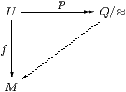
Proposition 15.11 From any open subspace U⊂ℝ
there is an open surjection p:U↠ Q/≈φ
with open connected fibres onto an overt discrete space.
Proof Let the subspace U be classified by φ:Σℝ without parameters. Let Q≡{a:ℚ ∣ φ a}⊂ ℚ, which is an open subspace of an overt discrete space, and therefore itself overt discrete (Proposition 11.16), and similarly ≈ restricts to a (total) open equivalence relation on Q. Hence the quotient Q/≈ is also an overt discrete space, and the map q:Q→ Q/≈ is an open surjection Section C 10.
By Theorem 10.2, the partial equivalence relation ≈ satisfies
| φ x =⇒ ∃ a.(x≈ a) and (x≈ a) ∧ (x≈ b) =⇒ (a≈ b), |
for a,b:ℚ. Hence, for x∈ U, x≈ a is a description that defines [a]:Q/≈, so there is a function p:U→ Q/≈ that makes the triangle commute:

The fibres of p are the equivalence classes of ≈, which are the open intervals that we obtained in Theorem 13.15. The map p goes from an overt space to a discrete one, and is therefore open Lemma C 10.2; it is surjective because q is.
Explicitly, by Axiom 7.10, an open subspace θ:ΣU is given by θ:Σℝ with θ⊑φ, so we define ∃pθ on the equivalence class [a]:A/(≈) by
| ∃pθ[a] ≡ ∃ b.(a≈ b)∧θ b. |
Then
| θ x =⇒ ∃ a.(x≈ a)∧θ a ≡ Σp(∃pθ) x. |
On the other hand, ψ:ΣQ/(≈) is given by ψ:Σℚ such that ψ a⊑φ a and (a≈ b)∧ψ b⇒ψ a, so
| ∃p(Σpψ)[a] ≡ ∃ b.(a≈ b)∧ψ b ⇔ ψ a. |
Hence ∃p⊣Σp and p is surjective. Finally,
| (ψ∧∃pθ)[a] ≡ ∃ b.ψ a∧θ b∧(a≈ b) ⇔ ∃ b.ψ b∧θ b∧ (a≈ b) ≡ ∃p(Σpψ∧θ)[a], |
which is the Frobenius law making p an open map. ▫
Lemma 15.12 The relation ≤ on Q/≈ defined by
| [x]≤[y] ≡ ∃ a,b:ℚ.x≈ a≤ b≈ y |
is a total but not necessarily decidable order, in the sense that
| [x]≤[x], [x]≤[y]≤[z]=⇒[x]≤[z], |
| [x]≤[y]≤[x]=⇒(x≈ y), [x]≤[y]∨[y]≤[x]. ▫ |
Theorem 15.13
Every open subspace U⊂ℝ is locally connected:
Proof The relation (x∼ y)≡(f x=M f y) is an open partial equivalence relation on ℝ with φ x⇒ x∼ x, so x≈ y⇒ x∼ y by Proposition 15.7. This means that f factors uniquely through the quotient Lemma C 10.8. The last part is the standard argument for universal properties: put the alternative candidate in the place of M to obtain the unique isomorphism. ▫
Local connectedness is studied in sheaf theory a parametric way by replacing the single overt discrete object M with a family of them indexed by some space A [JT84, §V.5].
Definition 15.14 A map m:M→ A is a local homeomorphism
or étale map if it is open,
the pullback or fibre product M×A M exists as a type
(cf. Section 7)
and the diagonal map M↪ M×A M is an open inclusion.
We have to make the existence of M×A M a hypothesis because
this construction has not yet been done in the ASD literature.
Theorem 15.15 The map p:U→ Q/(≈) is orthogonal
to any étale map m:M→ A.
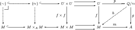
This means that, whenever we have a commutative square (g· p=m· f) as on the far right of the diagram above, there is a unique map h:Q/(≈)→ M that makes both triangles commute (f=h· p and g=m· h).
Proof All maps (≈)→ A in the diagram are equal, whilst M×A M↪ M× M⇉ A is an equaliser, so there is a fill-in (≈)→ M×A M. Then the inverse image (∼)↪(≈) of the open inclusion M↪ M×A M is an open total equivalence relation on U, so (∼)=(≈).
Symbolically, for x≈ z, we have p x=p z by construction of the quotient, and so a≡ m f x=g p x = g p z=m f z. Similarly, any x≤ y≤ z has x≈ y≈ z and so m f y=g p y=a too. This means that the interval [x,z] lies in the single fibre over a:A. The partial equivalence relation (y∼ y′)≡(f y=f y′) is defined in this fibre and is open because m:M→ A is étale, but it must be indiscriminate on the interval [x,z]. Thus (x≈ z)⇒(x∼ z)≡(f x=f z).
Since f respects the equivalence relation (≈), it factors through the quotient Q/(≈). ▫