


The topology that we shall impose on the topology of a space exploits the fact that the operators ▫ and ◊ preserve directed joins. It is now well known in theoretical computer science and topological lattice theory, so, if you are already familiar with either of these subjects, you may safely omit this section, as it just collects the basic facts of which you should be aware in order to follow the rest of the paper. Indeed, it serves as background and not an introduction, as our calculus will abstract from these ideas, rather than assume them.
In more traditional mathematical disciplines, on the other hand, the Scott topology is not as well known as it deserves, especially considering that it appears in real analysis in the guise of semicontinuity. The reason why it is absent from the curriculum is probably that it is not Hausdorff. Whilst there is a compact Hausdorff topology (the Lawson topology) that one can put on lattices of open sets, this does not have the properties that we require. The canonical textbook about these topologies and the continuous lattices on which they are particularly well behaved is [GHK++80]; its six authors represent the various disciplines in which these ideas arose.
Definition 3.1 Let L be any complete lattice.
A subset U⊂L is called Scott-open if
The Scott-open subsets form a topology on L. That is, ∅,L⊂L are Scott-open, if U,V⊂L are Scott-open then so is U∩V⊂L, and any union of Scott-open subsets is Scott-open.
It is crucial that you grasp the following point:
Exercise 3.2 Let L be the lattice of open subspaces of a locally compact space X.
Re-stating the usual “finite open sub-cover” definition
(Notation 2.14),
show that
a subset K⊂ X is compact iff the family
UK≡{U∈L ∣ K⊂ U} of open neighbourhoods of K
is a Scott-open subset of L.
▫
The compact–open topology on the set of continuous functions X→ Y was introduced by Ralph Fox in 1945 [Fox45]. Our topology is the much simpler special case in which Y is the Sierpiński space (Definition 3.8), but Dana Scott identified it as the crucial one in the study of topologies on function spaces [Sco72]. It had already become clear by then that the neighbourhoods of a compact subspace (which our ▫ and UK capture) are more important than its points [Wil70].
There are some other examples of the Scott topology that are useful in analysis and will play a major role in this paper. (In fact, they too can be seen as special cases of the topology on a topology on a space.)
Definition 3.3
The space ℝ of ascending reals consists,
| d∈ D ⇔ ∃ e:ℚ.d< e∈ D, |
and is endowed with the Scott topology that is defined by this order. The descending reals ℝ are defined in a similar way, but using the reverse arithmetical order, so U⊂ℚ is rounded upper if u∈ U⇔∃ t:ℚ.u> t∈ D. Arithmetic negation (−) takes descending reals to ascending ones and vice versa, indeed making ℝ≅ℝ, but it is not continuous as an endofunction of either space.
The significance of (this topology on) the space ℝ in traditional analysis is
Proposition 3.4
A function f:X→ℝ is lower semicontinuous
by definition if the inverse image of any open upper interval (d,+∞]
is open in X.
This happens iff f is continuous with respect to the Scott topology. ▫
So, when we say that all functions are continuous in our calculus, we are not precluding the consideration of semicontinuous functions: they just have to be seen as valued in ℝ or ℝ instead of in ℝ.
Example 3.5
The lower-semicontinuous step function
f:ℝ→ℝ⊂℘(ℚ)
may be defined by
| f x ≡ | ⎧ ⎨ ⎩ | d | ⎪ ⎪ ⎪ |
| ⎫ ⎬ ⎭ | . |
Notice that it takes the lower value at the steps.
Remark 3.6 Constructively, the spaces ℝ and ℝ
are not obtained by re-topologising the extended set of reals.
On the contrary, an ordinary Euclidean real number is defined
by a pair (called a Dedekind cut, cf. Definition 6.7)
consisting of an ascending real (the set of its rational lower bounds)
and a descending one (the upper bounds) that are compatible.
In the computable setting, there are descending reals that have
no ascending partner, and vice versa (Example 16.6).
The analysis of the ascending reals is very simple. In particular, any set of ascending reals has a supremum, given by union, and this is the limit of the set, so there is no difficulty with interchanging ascending limits, unlike two-sided ones.
These spaces offer two ways of forming the supremum of any set of Euclidean reals:
In our calculus, we will be able to form these two suprema when the set is compact or overt, respectively (Propositions 9.13 and 11.18).
Why should these two suprema be the same? Constructively, we need an additional condition on the set in order to ensure that the two parts define a Dedekind cut:
Definition 3.7
A subset K⊂ℝ obeys the
constructive least upper bound principle if
This condition, which is probably due to L.E.J. Brouwer, is necessary to form y≡supK because of the locatedness property (Axiom 4.9) of y with respect to (x< z), that is, it must satisfy either x< y or y< z. We shall find in Section 12 that this follows from the mixed modal laws (cf. Proposition 2.16) and is sufficient to define a Dedekind cut, and therefore a Euclidean real number.
You may perhaps think that this “constructive” situation is rather complicated, and could be simplified by adding some extra axioms. However, it is not difficult to adapt the arguments of Sections 1 and 16 to show that any such axiom would provide an oracle that could solve unreasonable computational and logical problems like those in Remark 1.3. We shall come to see that these anomalous situations are just as natural as singularities in polynomial equations, and are indeed closely related to them. When we recognise that ascending and descending reals occasionally lead their own separate lives, we come to appreciate the symmetries that real analysis enjoys, instead of its pathological counterexamples.
Definition 3.8
Our last example of the Scott topology is the Sierpiński space,
which we call Σ.
We define it as the lattice of open subspaces of the singleton.
Classically, therefore,
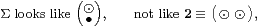
having two points and three open sets. We shall call these points ⊤ and ⊥, the former being open and the latter closed. Since Σ is a lattice, it also has ∧ and ∨.
The space 2 is both discrete and Hausdorff, but Σ is neither. Whilst there is a continuous function that takes the two points of 2 to those of Σ, any continuous function Σ→2 is constant. Hence Σ is connected, at least in the classical sense, and indeed in the constructive ones that we shall consider in Section 13. The map [0,1]→Σ by x↦(x> 0) even makes it path-connected.
This means that Σ has “more than” two points — there is something in between ⊥ and ⊤ that “connects” them. From a constructive point of view, this is because we defined the points of Σ as the open subsets of the singleton. There are more of these than just the decidable or complemented ones ⊥≡∅ and ⊤≡{⋆}.
The Sierpiński space was treated with derision in classical topology, but it is the spider in the middle of the web in our subject, being even more important than Proposition 3.4 for the ascending reals.
Proposition 3.9
For any space X, there is a bijective correspondence amongst
where we shall say that φ classifies U≡φ−1(⊤) and co-classifies C≡φ−1(⊥).
In particular, either U or C uniquely determines φ. ▫
Notice, therefore, that the correspondence between U and C is given by their common relationship to φ and not by set-theoretic complementation. This is how we avoid the double negations that appear frequently in work in the Brouwer and Bishop schools. Nevertheless, it is convenient to retain the word complementary for this relationship.
Remark 3.10
In the case where X≡Σ, continuous functions
Σ→Σ correspond to open subsets of Σ. Three of
these are definable: the identity and the constant functions
with values ⊥ and ⊤,
corresponding to the singleton, empty and entire open subspaces respectively.
Just as there was no arithmetical negation for the ascending reals
(Definition 3.3),
there is no continuous function (“logical negation”, ¬)
that interchanges ⊥ and ⊤.
More generally, Scott-continuous functions respect the order on the lattice. Indeed, any topological space X has a specialisation order, defined by
This is antisymmetric iff the space is T0, discrete iff it is T1 and (classically) it agrees with the order on the underlying lattice when that is given the Scott topology. Notice that we distinguish this order relation ⊑ from ≤ in real and integer arithmetic; they agree in the case of the ascending reals, but ⊑ is ≥ or = for the descending or Euclidean reals respectively. The key difference is that the order ⊑ is intrinsic, i.e. every continuous function f:X→ Y preserves it, whilst ≤ is imposed on ℕ, ℚ and ℝ, in the sense that continuous functions may in general preserve, reverse or ignore it.
Scott continuity is stronger than just preserving order, but instead of talking about arbitrary joins and finite sub-joins, it is convenient to introduce a new definition.
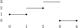
Definition 3.11 A poset (partially ordered set) (I,≤)
is directed if it is inhabited (has an element)
and, for any i,j∈I, there is some k∈I with i≤ k≥ j.
When we form a join or union indexed by I (taking ≤ to ⊑),
we use an arrow to indicate that it is directed: ⋁↑ or ⋃↑.
Examples 3.12 The following ordered sets are directed:
The Scott topology may be reformulated using directedness: U⊂L is open iff it is upper and, whenever ⋁↑ xi∈U, already xi∈U for some i∈ I. Hence this topology may be defined on any dcpo (directed-complete partial order), i.e. a poset in which every directed subset but not necessarily every finite subset has a join.
Proposition 3.13
A function F:L1→L2 between complete lattices (or dcpos)
is Scott-continuous, i.e. F−1(V) is Scott-open in L1
whenever V⊂L2 is Scott-open in L2,
iff F preserves directed joins, i.e.
| F(⋁i∈ I↑ xi) = ⋁i∈ I↑ F(xi) |
for all directed (xi)i∈ I⊂L1. Hence a function that is Scott-continuous in each of several variables is jointly continuous in them [Sco72, Props. 2.5&6]. ▫
Examples 3.14 Our operators ▫ and ◊ are Scott-continuous
functions from the lattice of open subspaces of X to Σ,
since they preserve directed joins (Notation 2.14).
Moreover, if they are defined in terms of some (function f with) parameters, they are jointly continuous with respect to both those parameters and to open subspaces of X, throughout the parameter space. By contrast, the Brouwer degree cannot be continuous at singularities, because of the fact that it takes values in ℤ.
Remark 3.15
The use of directed covers of compact spaces
instead of general ones simplifies the idioms of analysis,
because covers are often naturally indexed by the rationals or reals.
Suppose, for example, that we want to find an upper bound for a function f:K→ℝ. The subsets Uu≡{k∈ K ∣ f k< u} indexed by candidate bounds u∈ℚ are open and cover K, so only finitely many of them are needed. Now, u ranges over a (totally ordered and so) directed poset ℚ, and we have u≤ v⇒ Uu⊂ Uv. Therefore the finite open sub-cover need only have one member, named by the greatest u in the finite set, and we have K⊂ Uu for a single u. In other words, there is a uniform bound.
More abstractly, a directed family (Uu) that respects the order on u∈ℚ corresponds to an upper semicontinuous function f:K→ℝ, and to a directed relation θ, by
| (k∈ Uu) ≡ θ(k,u) ≡ (f k< u). |
When we need to state Scott continuity in our abstract calculus, in Section 9, it will be most convenient to formulate it using θ, which must satisfy
| (u≤ v) ∧ θ(k,u) =⇒ θ(k,v). |
This situation also arises with the opposite order. For example, in the definitions of continuity and differentiability (Section 10) we require δ> 0 with a certain property. Underlying this is a lower semicontinuous function, a directed family of subsets with δ≤ε⇒ Uδ⊃ Uε, or a relation θ that satisfies
| (δ≤ε) ∧ θ(k,ε) =⇒θ(k,δ). |
Now let’s think about Proposition 3.9 again.
Notation 3.16 Since open sets U⊂ X correspond to
continuous maps X→Σ, we write ΣX for the lattice of
them, equipped with the Scott topology.
This correspondence also gives rise to the notation
| φ a or φ a⇔⊤ for a∈ U |
for membership of this subspace.
Implicit in the expression “φ a” is a binary higher-type function, called evaluation or application, so ev(φ,a)≡φ a. We want this, like everything else, to be continuous, but this requirement places a severe restriction on the compatibility of the ideas in this paper with those of traditional topology:
Proposition 3.17
The function ev:ΣX× X→Σ
is jointly continuous (with respect to the Tychonov product topology
defined from the given topology on X and the Scott topology on ΣX
and Σ) iff X is locally compact
[GHK++80, Thm. II 4.10], [Joh82, §VII 4]. ▫
As we are dealing with non-Hausdorff spaces (in particular ΣX) here, we need to adjust the traditional definition of local compactness [HM81]:
Definition 3.18 A (not necessarily Hausdorff) space X is
locally compact if, whenever x∈ U⊂ X with U open,
there are compact K and open V with x∈ V⊂ K⊂ U.
This relation between open subsets, written V≪ U and called way below, may be characterised without mentioning the compact subspace K between them: if U⊂⋃↑ Wi then already V⊂ Wi for some i. This is the point from which the theory of continuous lattices begins [GHK++80], but we shall not need to make much use of it, beyond observing the ubiquitous alternating inclusions of open and compact intervals in real analysis (Remark 10.1).
The result that justifies calling ΣX a function-space is then
Theorem 3.19
Let X be locally compact and Γ any space.
Then ΣX is also locally compact
and there is a bijection between continuous functions
| Γ× X —→ Σ and Γ—→ ΣX |
that is given in the backward direction by composition with ev:ΣX× X→Σ. This correspondence is natural in the space Γ, i.e. it respects pre-composition with any continuous function Δ→Γ [Sco72, Section 3]. ▫
Remark 3.20
Dana Scott’s work grew into the two disciplines of domain theory and
denotational semantics in theoretical computer science,
giving topological meanings to programs as continuous functions.
These ideas are particularly useful for functional programming languages,
i.e. those in which functions may be defined as first class objects,
e.g. [Plo77].
Functions are interpreted using λ-abstraction,
whilst recursive definitions that need not necessarily terminate
or be well founded are given a meaning in terms of directed joins.
Denotational semantics was founded on an intuition of the analogy between continuity and computation that had earlier roots in recursion theory such as the Rice–Shapiro theorem [Ric56]. In particular, the recursively enumerable subsets of ℕ provide something like a topology, in so far as they admit all finite intersections and some infinite unions.
The connection can be put more simply than this, in terms of computation with real numbers. We cannot make a positive (terminating) test for equality (cf. Remark 1.3), but we can do so for ≠, > or <. More generally, we may observe membership of an open subspace, since that is determined by some finite approximation to (essentially, finitely many decimal places of) the number. Like open subsets, (parallel) observations admit finite intersections and (some) infinite unions. Another basic intuition of Scott continuity is that the result of a computation depends on only a finite part of the data.
We shall begin the axiomatisation of our calculus in the next section from these remarks, but first we need to make some more foundational observations about general topology.
Remark 3.21
The Sierpiński space is particularly familiar in computation,
because it provides the type of values of a program that may terminate (⊤)
or diverge (⊥) but generates no numerical output or other side-effect.
This type is called void in C and Java.
An input of this type is a signal that may or may not ever
arrive.
Then a program F of type Σ→Σ, i.e. which takes a signal as input and then may terminate (output another signal) or diverge, may behave in one of three ways:
The one thing that it cannot do is to negate its input (¬), i.e. terminate iff its signal never arrives; this is called the Halting problem [Tur35]. The type Σ is therefore quite different from a two-element or Boolean type.
This situation is the same as that in Remark 3.10, except that we are now able to see computationally something that was perhaps a little ambiguous in constructive topology, namely the general behaviour of any program F:Σ→Σ is determined by the specific cases F⊤ and F⊥ in which it definitely does or does not receive the signal.
As in topology, we must have F⊥⊑ F⊤, i.e. if the program terminates without receiving the input signal, it must also terminate if it does receive it (for example, the signal might arrive just after F has terminated).
Using the lattice structure on Σ, we may use “linear interpolation” to define a function F:Σ→Σ, from F⊤ and F⊥. Because of the previous remark, this recovers the original F:
Definition 3.22
The Phoa principle (pronounced “Pwah”) [Hyl91]
says that
| for any F:Σ→Σ and x:Σ, Fx ⇔ F⊥∨ x∧ F⊤. |
It would be wise to pause for a moment’s reflection on the ways in which we have motivated the Phoa principle in topology (Remark 3.10) and computation. This is the key step in the abstraction that we shall make in ASD, because it is exactly the condition that is required to ensure the extensional correspondence amongst open and closed subspaces and terms of type ΣX in Proposition 3.9 [C].
It will also provide the glue that gives our proofs their coherence. However, the rules of inference in topology to which it leads (Axiom 5.6) may appear to be classical, so we emphasise that it was discovered as a result of investigations in several constructive disciplines.
One of these is locale theory, which is a formulation of general topology purely in terms of lattices, without mentioning points; Peter Johnstone’s book [Joh82] is an outstanding account of this and its relationship to many areas of mathematics, in particular analysis. The validity of our principle for locales is shown in Paragraph O 7.5, but it had been noticed independently as the so-called Frobenius laws for open [JT84] and proper [Ver94] maps, cf. Propositions 11.2 and 8.2 respectively.
As for its connection with real analysis, the Phoa principle is similar to Markov’s principle, but the historical links involve too many unrelated ideas along the way to give the bibliographical trail.
Remark 3.23 There is a certain imprecision about the analogy between
topology and recursion theory, since the former traditionally requires
arbitrary unions, but the latter only recursive ones.
In fact, the translation from programs to continuous functions
is perfectly rigorous and has been used very successfully to develop
methods of demonstrating correctness of programs.
One may also try to reformulate topology using σ-frames,
i.e. lattices with countable unions, over which meets distribute
(the σ follows the usage of probability theory,
but it is confusing in our notation).
However, countability is just a mutilated form of set theory
that does not get to grips with computation
and actually makes no difference for objects such as ℕ and ℝ.
These issues may be addressed by considering topology and computation in parallel, i.e. by requiring the morphisms to be pairs consisting of a continuous function and a program that “agree” in a suitable sense. There are two such techniques that are well established. One uses logical relations and can show that, if the topological denotation of a program is ⊤ then its computation terminates [Plo77], cf. Remark 6.6. The other, called type two effectivity, develops computational representations of many ideas in classical general topology and real analysis [Wei00].
We have already seen in Proposition 2.12 that our possibility operator ◊ and the new notion of overtness are badly represented by the arbitrary unions of subsets that are used in traditional general topology. We want to replace these arbitrary unions by recursive ones, thereby legitimising the idea that the RE subsets of ℕ form a topology (Remark 3.20). However, when we consider how complicated both topology and recursion theory are on their own, it seems to be a recipe for a dog’s breakfast to try to combine them into a new theory.
So that’s not what we are going to do: the revolutionary approach that we shall follow in this paper is quite different from any of these things. We begin by abandoning traditional topology and recursion theory altogether, and returning to some extremely basic intuitions about the things that we can calculate about real numbers. We find that, without ever introducing set theory, we can recover the main results about continuity on the real line, including the issues regarding connectedness and solutions of equations that we introduced in the first two sections. On the other hand, it has been well known since the time of Alonzo Church, Stephen Kleene and Alan Turing that more or less anything that looks like computation is equivalent to the standard forms (at least as far as partial functions from ℕ to ℕ are concerned). In particular, there are already enough ingredients amongst our topological ideas to do general computation.
Overtness plays a key role underlying all of this. In the previous section, we saw manifestations of it in open maps, the existential quantifier and the join-preserving property of ◊. It is also related to recursive enumerability, and specifies which joins exist in open set lattices and the ascending reals. However, despite the fact that it does so many jobs, we don’t have to do anything to encode this behaviour into the system: it will all just fall out naturally.
In this section we have introduced some ideas from non-Hausdorff general topology because they underlie four decades’ work in the theory of computation but are largely unknown to those mathematicians who do not work in computer science departments. In particular, they provide the background for our new calculus. However, I now ask you to forget them again, along with all of the other textbook accounts of general topology, and begin the next section with a fresh mind. Our new calculus will “stand on its own feet”. It has a concrete representation that we have just sketched, but is not defined by it, just as groups may be represented by permutations or matrices, and integers by sheep or pebbles. Progress in mathematics is made by abstraction from such things, leaving the old concrete form behind.