


Although we have used completely coprime filters to introduce sobriety, we shall not use lattice theory in the core development in this paper, except to show in Section 5 that various categories of topological spaces and continuous functions provide models of the abstract structure.
We shall show instead that sobriety has a new characterisation in terms of the exponential Σ(−) and its associated λ-calculus. The abstract construction in Sections 3, 4, 6, 7 and 8 will be based on some category C about which we assume only that it has finite products, and powers Σ(−) of some special object Σ. In most of the applications, especially to topology, this category is not cartesian closed: it is only the object Σ that we require to be exponentiating. [See1 Remark C 2.4 for discussion of this word.]
This structure on the category C may alternatively be described in the notation of the λ-calculus. When C is an already given concrete category (maybe of topological spaces, domains, sets or posets), this calculus has an interpretation or denotational semantics in C. Equally, on the other hand, C may be an abstract category that is manufactured from the symbols of the calculus. The advantage of a categorical treatment is, as always, that it serves both the abstract and concrete purposes equally well.
Definition 2.1
The restricted λ-calculus has just the type-formation rules
1 type
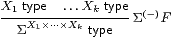
|
but with the normal rules for λ-abstraction and application,
|
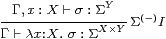
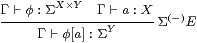
together with the usual α, β and η rules B 9.1, ΣY× Z=(ΣZ)Y.
The turnstile (⊢) signifies a sequent presentation in which there are all of the familiar structural rules: identity, weakening, exchange, contraction and cut.
Remark 2.2 As this is a fragment of the simply typed λ-calculus,
it strongly normalises.
We shall take a denotational view of the calculus,
in which the β- and η-rules are
equations between different notations for the same value,
and are applicable at any depth within a λ-expression.
(This is in contrast to the way in which λ-calculi are made to
agree with the execution of programming languages, by restricting the
applicability of the β-rule [Plo75].
Besides defining call by name and call by value
reduction strategies, this paper used continuations to interpret one
dually within the other.)
Notation 2.3 We take account of the restriction on type-formation
by adopting a convention for variable names:
lower case Greek letters and capital italics
denote terms whose type is (a retract of) some ΣX.
These are the terms that can be the bodies of λ-abstractions.
Since they are also the terms to which the lattice operations and ∃
below may be applied, we call them logical terms.
Lower case italic letters denote terms of arbitrary type.
As we have already seen, towers of Σs like ΣΣX tend to arise in this subject. We shall often write Σ2 X, and more generally Σn X, for these. (Fortunately, we do not often use finite discrete types, but when we do we write them in bold: 0, 1, 2, 3.) Increasingly exotic alphabets will be used for terms of these types, including
| a,b,x,y:X φ,ψ:ΣX F,G:ΣΣX F,G:Σ3 X. |
Remark 2.4
In order to model general topology (Section 5)
we must add the lattice operations ⊤, ⊥, ∧ and ∨,
with axioms to say that Σ is a distributive lattice.
In fact, we need a bit more than this.
The Euclidean principle,
| φ:Σ, F:ΣΣ ⊢ φ∧ F(φ) ⇔ φ∧ F(⊤), |
captures the extensional way in which ΣX is a set of subsets [C]. It will be used for computational reasons in Proposition 10.6, and Remark 4.11 explains why this is necessary.
Remark 2.5
We shall also consider the type ℕ of natural numbers,
with primitive recursion at all types, in
Sections 9–10
(where the lattice structure is also needed).
Terms of this type are, of course, called numerical.
Note that ℕ is a discrete set, not a domain with ⊥.
Strong normalisation is now lost.
The notation that we use for primitive recursion at type X is
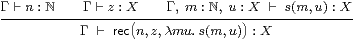
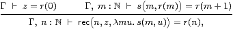
|
where Γ and m:ℕ are static and dynamic parameters, and u denotes the “recursive call”. The β-rules are
| rec(0, z, λ m u.s)=z rec(n+1,z,λ m u.s)=s(n,rec(n, z, λ m u.s)). |
Uniqueness of the rec term is enforced by the rule
|
whose ingredients are exactly the base case and induction step in a traditional proof by induction. [In fact we need to allow equational hypotheses in the context Γ, see Remark E 2.7.]
Countable joins in ΣΓ may be seen logically in terms of the existential quantifier
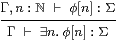
|
for which distributivity is known as the Frobenius law.
Remark 2.6 For both topology and recursion,
a further axiom (called the Scott principle in [Tay91])
is also needed to force all maps to preserve directed joins:
| Γ, F:Σ2ℕ ⊢ F(λ n.⊤) ⇔ ∃ n.F(λ m.m< n). |
For any Γ⊢ G:ΣX→ΣX, let Γ ⊢ Y G = ∃ n.rec (n,λ x.⊥, λ m φ.Gφ) :ΣX and
| Γ, x:X ⊢ F = λφ.G(∃ n.φ n∧ rec (n,λ x.⊥, λ m φ.Gφ))x. |
Then F(λ n.⊤) ⇔ G(Y G)x and ∃ n.F(λ m.m< n) ⇔ Y G x, so Y G is a fixed point of G, indeed the least one. However, this axiom is not needed in this paper, or indeed until we get rather a long way into the abstract Stone duality programme [F][G].
Remark 2.7 We shall want to pass back and forth
between the restricted λ-calculus and the corresponding
category C. The technique for doing this fluently is a major theme
of [Tay99]; see Sections 4.3 and 4.7 in particular.
When a sequent presentation such as ours has all of the usual structural rules (in particular weakening and contraction), there is a category with products
We shall not need the notation ↑ x in this paper, but we shall re-use the . for a different purpose in Section 6. (There we also introduce a category HC that does not have products, but, unlike other authors, we shy away from using a syntactic calculus to work in it, because such a calculus would have to specify an order of evaluation.)
Proposition 2.8 The category C so described is
the free category with finite products and an exponentiating object
Σ, together with the additional lattice and recursive structure
according to the context of the discussion.
Proof The mediating functor ⟦−⟧:C→D from this syntactic category C to another (“semantic”) category D equipped with the relevant structure is defined by structural recursion. ▫
The exponentiating object Σ immediately induces certain structure in the category.
Lemma 2.9 Σ(−) is a contravariant functor.
In particular, for f:X→ Y, ψ:ΣY and F:Σ2 X, we have
| Σf(ψ)=λ x.ψ[f x] and Σ2 f(F)=λ ψ.F(λ x.ψ[f x]). |
Proof You can check that Σid=id and Σf;g=Σg;Σf. ▫
In general topology and locale theory it is customary to write f*ψ⊂ X for the inverse image of ψ⊂ Y under f, but we use Σfψ instead for this, considered as a λ-term, saving f* for the meta-operation of substitution (in Lemmas 8.7 and 9.2).
Now we can describe the all-important neighbourhood-family ηX(x) (Remark 1.4) in purely categorical terms. As observed in [Tay99, Remark 7.2.4(c)], it is most unfortunate that the letter η has well established meanings for two different parts of the anatomy of an adjunction.
Lemma 2.10 The family of maps ηX:X→ΣΣX,
defined by x↦(λ φ.φ x),
is natural and satisfies ηΣX;ΣηX=id
(which we call the unit equation).
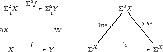
Proof As this Lemma is used extremely frequently, we spell out its proof in the λ-calculus in detail. Using the formulae that we have just given,
| Σ2 f(ηX x)= λψ.(λφ.φ x)(λ x′.ψ(f x′))= λψ.(λ x′.ψ(f x′))(x)=λ ψ.ψ(f x)=ηY(f x). |
Also, ΣηX(F)=λ x.F(ηX x)=λ x.F(λ φ.φ x) for F:Σ3(X), so
| ΣηX(ηΣ Xφ) =λ x.(λ F.Fφ)(λφ′.φ′ x)= λ x.(λ φ′.φ′ x)(φ) =λ x. φ x = φ. ▫ |
Proposition 2.11
The contravariant functor Σ(−)
is symmetrically adjoint to itself on the right,
the unit and counit both being η.
The natural bijection

|
defined by P=ηΓ;ΣH and H=ηX;ΣP is called double exponential transposition.
Proof The triangular identities are both ηΣX;ΣηX=id. ▫
Remark 2.12
The task for the next three sections is to characterise,
in terms of category theory, lambda calculus and lattice theory,
those P:ΣΣX that (should) arise as ηX(a)
for some a:X.
The actual condition will be stated in Corollary 4.12, but, whatever it is, suppose that the morphism or term
| P:Γ→ΣΣX or Γ⊢ P:ΣΣX |
does satisfy it. Then the intuitions of the previous section suggest that we have defined a new value, which we shall call
| Γ⊢focusP:X, |
such that the result of the observation φ:ΣX is
| Γ ⊢ φ(focusP) ⇔ Pφ : Σ. |
In particular, when P≡ηX(a) we recover a=focusP and φ a ⇔ Pφ. These are the β- and η-rules for a new constructor focus that we shall add to our λ-calculus in Section 8.
Remark 2.13 In the traditional terminology of point-set topology,
a completely coprime filter converges to its limit point,
but the word “limit” is now so well established with a completely different
meaning in category theory that we need a new word.
Peter Selinger [Sel01] has used the word “focus” for a category that is essentially our SC. The two uses of this word may be understood as singular and collective respectively: Selinger’s focal subcategory consists of the legitimate results of our focus operator.
We now turn from the type X of values to the corresponding algebra ΣX of observations, in order to characterise the homomorphisms ΣY→ΣX that correspond to functions X→ Y, and also which terms P:ΣΣX correspond to virtual values in X.