


Paré’s theorem, that any elementary topos has the monadic property [Par74], which originally inspired abstract Stone duality, was itself motivated by the simple way that it affords for constructing colimits. So we conclude this paper with applications of the comprehension calculus to coproducts and coequalisers.
Example 11.1 The idea of Stone duality is to consider spaces
in terms of the corresponding algebras.
For any algebra (A,α), we have
| pts(A,α) ≡ {ΣA ∣ ηA·α≡λ Fφ.φ(α F)}, |
in which ηA·α is a nucleus (Definition 8.7) because of the Eilenberg–Moore equations for α. The homomorphism H:B→ A corresponds to the function
| x:pts(A,α) ⊢ admit(λψ.Hψ(i x)):pts(B,β), |
in which H is behaving as a continuation-transformer. (We saw in the previous section that the operators i and admit merely serve as compile-time type-annotation.) In particular, if H≡Σf, where f:X→ Y, this is just focus(λψ.ψ(f x)) = f x by Lemma 8.11. ▫
The continuation-passing style is more clearly visible in a more complicated example.
Example 11.2 The coproduct X+Y of spaces corresponds to the product
A≡ΣX×ΣY of algebras,
whose structure map α≡<P0,P1> was given in Lemma 5.5:
| P0:Σ2(ΣX×ΣY)→ΣX by H↦λ x.H (λφψ.φ x). |
Then X+Y ≡ pts(A,α) ≡ {ΣΣX×ΣY ∣ EX+Y}, where
| EX+Y ≡ ηΣX×ΣY·α:H↦λ H.H <P0H, P1H>. |
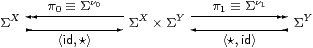
The inclusion ν0:X→ X+Y satisfies Σν0= π0, so
| ν0(x)≡ admit(λφψ.φ x) and ν1(y)≡ admit(λφψ.ψ y). |
Then, for f:X→ Z and g:Y→ Z, the mediator X+Y→ Z is
| [f,g]:u↦ focus(λθ. (i u)(λ x.θ(f x))(λ y.θ(g y))), |
in which the continuation θ from Z is passed either as θ· f to X or as θ· g to Y. When u≡ ν0(x) or ν1(y), one of the two branches is selected and that continuation is applied to x or y. ▫
We already know that products distribute over coproducts (Proposition A 7.11), and coproducts are disjoint and stable under pullback on the assumption that Σ is a distributive lattice and satisfies the Euclidean principle (Section C 9). In fact this extra structure is unnecessary: if (S,Σ) is monadic then S is extensive on a very much weaker assumption.
[The initial object 0 is strict (X×0≅0) by sobriety, because
| ΣX×0 ≅ (Σ0)X ≅ 1X ≅ 1 ≅ Σ0. |
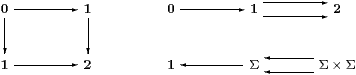
For disjointness of coproducts, the square is a pullback iff the upper right diagram is an equaliser. By monadicity, this happens iff the lower right diagram is a coequaliser, which it is iff Σ↠1 is regular epi.
The following results are based on the stronger assumption that this map is split epi, which it is in topology. It seems unlikely that any other application would require the weaker hypothesis.]
Lemma 11.3 The map 0→1 is a Σ-split mono iff
Σ has a constant.
Proof I:Σ0≡ 1→Σ≡ Σ1. ▫
If I≡ ⊤, this makes 0 a closed subspace; if I≡ ⊥ then it’s open (Examples 2.5). However, we shall call the constant ⋆ here to emphasise that we are not using any lattice structure. Then coproduct inclusions are also Σ-split monos:
Lemma 11.4 X≅{X+Y ∣ <π0,⋆>} and
Y≅{X+Y ∣ <⋆,π1>}.
Proof These idempotents arise from the diagram
▫
We want to show that every map U→2 arises in this way from a unique coproduct. Because of the continuation-passing behaviour, it is convenient to treat 2 as a subspace of ΣΣ×Σ. Then the definable elements are π0≡λ x y.x and π1≡λ x y.y, which simply select the appropriate continuation from the pair.
Lemma 11.5 2 ≅
{ΣΣ×Σ ∣ λF F.F(Fπ0,Fπ1)}.
Proof This is the primality equation, F P ⇔ P(λ x.F(λφ.φ x)), with λ x replaced by the two values 0,1:2, and φ:Σ2 by a pair. ▫
We shall abuse our language by calling the two-argument functions P:ΣΣ×Σ that belong to this subspace “prime”. However, we need yet another characterisation of them.
Lemma 11.6 Γ⊢ P:ΣΣ×Σ is prime iff,
for x,y,z:Σ and G:ΣΣΣ,
| P(x,x) ⇔ x P(P(x,y),z) ⇔ P(x,z) ⇔ P(x,P(y,z)) |
| G(λ z. P(z,⋆)) ⇔ P(Gid, G(λ z.⋆)) G(λ z. P(⋆,z)) ⇔ P(G(λ z.⋆), Gid). |
Proof If P is prime, so Γ, F:Σ2(Σ×Σ) ⊢ F P ⇔ P(Fπ0,Fπ1), then
The converse is not needed in the following applications.
We first put G≡λθ.F(λ x y.θ P(x,y)), so
G(λ z.⋆) ⇔ F(λ x y.⋆), Gid ⇔ F P,
| G(λ z.P(z,⋆)) ⇔ F(λ x y.P(P(x,y), ⋆)) ⇔ F(λ x y.P(x,⋆)), |
| G(λ z.P(⋆,z)) ⇔ F(λ x y.P(⋆,P(x,y))) ⇔ F(λ x y.P(⋆,y)), |
with which the equations involving G give
| F(λ x y.P(x,⋆)) ⇔ P(F P, F(λ x y.⋆)) F(λ x y.P(⋆,y)) ⇔ P(F(λ x y.⋆), F P). |
Next put G≡ λθ.F(λ x y.θ x), so
| G(λ z.⋆) ⇔ F(λ x y.⋆), G(λ z.P(z,⋆)) ⇔ F(λ x y.P(x,⋆)) and Gid ⇔ Fπ0, |
with which the first G-equation gives
| F(λ x y.P(x,⋆)) ⇔ P(Fπ0, F(λ x y.⋆)), |
and similarly G≡ λθ.F(λ x y.θ y) yields F(λ x y.P(⋆,y)) ⇔ P(F(λ x y.⋆), Fπ1).
From these four consequences of the higher-type G-equations, together with the ones of base type, we deduce that P is prime:
|
Proposition 11.7
Let u:U⊢ P u:ΣΣ×Σ be prime.
Then the following subspaces are well defined, their coproduct is U
and the squares are pullbacks.
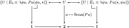
Proof To show that E0 is a nucleus, we must show for u:U and F:Σ3 U that
| E0(λ v.F(λφ.E0φ v)) u ⇔ P u(F(λφ.P u(φ u,⋆)), ⋆) ≡ P u(y,⋆) |
is equal to
| E0(λ v.F(λφ.φ v)) u ⇔ P u(F(λφ.φ u), ⋆) ≡ P u(x,⋆). |
Put G≡λθ.F(λφ.θ(φ u)) in the Lemma. Then
|
so P u(y,⋆) ⇔ P u(P u(x,t),⋆) ⇔ P u(x,⋆) as required.
To test that the left hand square is a pullback, we are given Γ⊢ v:U such that Γ⊢ P v=π0. Then
| Γ, θ:ΣU ⊢ E0θ v ⇔ P v(θ v,⋆) ⇔ π0 (θ v,⋆) ⇔ θ v, |
as is required to form the mediator Γ⊢ admitv:{U ∣ E0}.
To show that U is the coproduct, we must show that ΣU is the associated product, i.e. that θ:ΣU corresponds bijectively to <φ,ψ> where φ=E0φ and ψ=E1ψ. In fact, P serves for the pairing operation as well as for the projections: θ≡λ u.P u(φ u,ψ u).
| θ ↦ <λ u.P u(θ u,⋆), λ u.P u(⋆,θ u)> ↦ λ u.P u(P u(θ u,⋆), P u(⋆,θ u)) = λ u.θ u |

▫
Theorem 11.8
If (S,Σ) is monadic and Σ has a constant
then S is extensive, i.e. it has stable disjoint coproducts
[Tay99, Section 5.5].
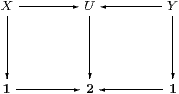
Proof We have to show that the commutative diagram is a pair of pullbacks iff its top row is a coproduct. The map U→2 must arise from a prime u:U⊢ P u:ΣΣ×Σ, from which Proposition 11.7 constructs subspaces forming pullbacks and a coproduct. Since pullbacks are unique up to isomorphism, if the given diagram is a pair of pullbacks then it is isomorphic to that in the Proposition.
Conversely, if we are given a coproduct U≡ X+Y then u:U⊢ P u:ΣΣ×Σ is defined by x:X⊢ P x≡π0 and y:Y⊢ P y≡π1. Then E0 in the Proposition becomes
| E0θ = E0<φ,ψ> = <λ x.π0<φ,ψ> x, λ y.⋆> = <φ,⋆>, |
which agrees with Lemma 11.4. ▫
Corollary 11.9 Let x:X⊢ f x,g x:Z and
x:X⊢ P x:ΣΣ×Σ with P prime. Then
| if (focusP) then f x else g x = focus(λθ. P x (θ(f x)) (θ(g x))). ▫ |
Turning from coproducts to coequalisers, of course we can only construct those that are Σ-split. We leave the reader to formulate Beck-style equations as in Section 3, concentrating instead on the analogue for quotients of the comprehension calculus for subspaces in Section 8. Beware also that the class of Σ-epis is stable under products but not necessarily pullbacks. For the topological motivation, recall that the quotient topology on a set Y induced by the function q:X→ Y from a topological space has V⊂ Y open iff q−1V is open in X.

be a Σ-split epi, and put R≡Q· q. Then
| Y ≅ {Σ2 X ∣ E}, where EF F ≡ F(λ x.F(λφ.R φ x)), |
| q x = admit(λφ. Rφ x) and Q φ = λ y. i yφ. |
Proof Three of the four squares
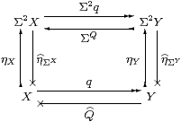
commute by naturality, but that from Y to Σ2 X need not. So E is the composite from Σ2 X anticlockwise back to itself:
| ≡ Σ2 q; |
| ΣY; ηY;ΣQ = |
| ΣX; q; ηY; ΣQ = |
| ΣX; ηX; ΣΣq; ΣQ, |
so EF F ⇔ ηΣX(ΣηX(Σ2 R F)) F ⇔ F(λ x.F(λφ. Rφ x)). Next,
| i(q x) = ΣQ(ηY(q x)) = ΣQ(Σ2 q(ηX x)) = ΣR(ηX) = λφ. Rφ x, |
whence q x = admit(λφ. Rφ x). Finally, i yφ = ΣQ(ηY y)φ = (λφ. φ y)(Qφ) = Qφ y. ▫
Proposition 11.11
Y≡ X/R , q x ≡ [x] and
| (let y=[x] in f x) ≡ focus(λθ.Q(θ· f)y) ≡ focus(λθ.(i y)(θ· f)) |
satisfy the rules
| x:X ⊢ [x]:X/R /I |
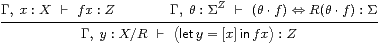 /E
/E
|
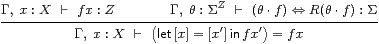 /β
/β
|
| y:X/R ⊢ (let y=[x] in [x]) = y /η, |
together with those for the quotient topology (Σ/ I, Σ/ E, Σ/ β and Σ/ η),
|
Proof We verify the /β and /η rules:
|
Remark 11.12 Notice that the β-rule is not a computational
reduction, but a denotational equation that is a consequence
of the equation R(θ· f)=(θ· f) in its hypothesis.
A compiler equipped with a proof assistant might perhaps
be able know this, but otherwise we can only hope that the implementation
will somehow find its way from one side of the β-rule to the other.
Let us specialise this to sets and (discrete) topological spaces, now making use of the lattice structure.
Example 11.13 Section C 10 constructs
the quotient X/δ of an overt discrete object X
by the open equivalence relation classified by δ:X× X→Σ.
Overt discrete means that X is equipped with predicates
∃X:ΣX→Σ and (=X):X× X→Σ
satisfying the usual properties.
The construction in Lemma C 10.8 obtains ΣX/δ (which is unfortunately called ΣQ=E there, for “quotient” and “equaliser”) as a retract of ΣX, namely as the image of the closure operation
| R ≡ Σq·∃q ≡ λφ x.∃ y.δ(x,y)∧φ(y). |
The quotient space is therefore X/δ=X/R={Σ2 X ∣ E}, where
|
If f:X→ Z respects the equivalence relation δ then the β-rule is
| focus(λθ.∃ y.δ(x,y)∧θ(f y)) = f x. |
In principle this computation involves a search of the equivalence class, which makes sense, given the connection between coequalisers and while programs [Tay99, Section 6.4].
Example 11.14 As explained in Remark C 10.12,
there is another representation of X/δ that is more like
the familiar one with equivalence classes.
It arises from the factorisation

of the transpose of the equivalence relation. This generalises
| ℕ ≅ {Σℕ ∣ E} by n↦ |
| , where E ≡ λ Fφ.∃ n.F(λ m.m=n)∧φ n, |
cf. Section A 10. The quotient is now given by {ΣX ∣ E}, where
| E ≡ λ Fφ.∃ x.F(λ y.δ(x,y))∧φ x, |
with q x ≡ admit(λ y.δ(x,y)).
If f:X→ Z respects the equivalence relation then the mediator X/δ→ Z is
| y ↦ focus(λθ.∃ x′.i y x′∧θ(f x′)). |
This selects an element x′ from the equivalence class y∈ X/δ (classified by a predicate i y∈ΣX) and applies f to it, as we would expect. Substitution of y ≡ q x yields the same formula focus(λθ.∃ x′.δ(x,x′)∧θ(f x′)) as before. ▫
Remark 11.15 Here is a summary of the comprehension types that we have used.
|