


In this paper we develop a computable account of locally compact sober spaces and locales, but using a λ-calculus in place of the usual infinitary lattice theory, which conflicts with computable ideas. This calculus, called Abstract Stone Duality, exploits the fact that, for any such space X, its lattice of open subspaces provides the exponential ΣX in the category. Here Σ is the Sierpiński space (which, classically, has one open and one closed point), and the lattice ΣX is equipped with the Scott topology. Its relationship to the “consistency conditions” in the previous sections and in [JS96] will be examined in Sections 11–16.
In this section and the next we present the axiomatisation of ASD in a reflective fashion that is intended to examine the reasons for our choices. For a straightforward summary of the calculus intended for applications, see [I] instead.
Remark 3.1
We are primarily interested in two particular models of the calculus:
The classical side has a wealth of concepts motivated by geometry and analysis, but its traditional foundations are logically very strong, being able to define many functions that are neither continuous nor computable, besides many other famous pathologies. Having created such a wild theory, we have to rein it back in again, with a double bridle. The topological bridle is constructed with infinitary lattice theory, whilst in recursion theory we are reduced to using Gödel numberings of manipulations of codes for basic elements. Abstract Stone duality avoids all of this by only introducing computably continuous functions in the first place. (We pay a logical price for this in not being able to define objects and functions anything like so readily as in set theory.)
On the other hand, logically motivated discussions often read the foundational aspects more literally than their topological authors ever intended. They are so bound up in their own questions of what constitutes “constructivity” that they lose sight of the conceptual structure behind the mathematics itself. For one example, in several constructive approaches to topology, the closed real interval fails to be compact. For another, whilst the mathematician in hot pursuit of a proof typically postulates a least counterexample, in order to rule it out, it is impertinent of the logician to emphasise that this uses excluded middle, since proofs of this kind (once found) can very often be recast in terms of the induction scheme [Tay99, Section 2.5]. As a result, foundational work often fails to reach “ground level” in the intended construction.
The lesson that we draw from this is that logic and topology readily drift apart, if ever we let go of either of them for just one moment. So we have to tell their stories in parallel. This means that we must often make do with rough-and-ready versions of parts of one, in order to make progress with the other. For example, we use concepts such as compactness to motivate our λ-calculus, which itself underlies the technical machinery that eventually justifies the correspondence with traditional topology and the use of its language. We shall make a point of explaining how each step (Definition, Lemma, etc. ) of the new argument corresponds to some idea in traditional topology.
This means that you will have to be prepared for some sudden switches between contexts. This paper is highly experimental. It introduces λ-calculus formulations of topological concepts and arguments, which it has to try out in the traditional categories for topology, even though these are defective for the purpose. When we are sure that we have all of the axioms in place (which was certainly not the case before this investigation began, but is close to being so after it) the best way to handle the relationship will not be to interpret ASD in locale theory, but vice versa [H].
In this section we have to set up some logical structure to which the topologically minded reader may prefer to return after first reading Section 6. We catch up on some of the justifications in Sections 9 and 10, for example characterising our morphisms in terms of preservation of meets and joins. In this section too, we interleave the axioms and definitions of the λ-calculus with the technical issues that they are intended to handle.
Remark 3.2
Recall first the universal properties of the Sierpiński space, Σ.
Any open subspace U⊂ X is classified
by a continuous function φ:X→Σ,
in the sense that U=φ−1(⊤),
where ⊤ is the open point of Σ,
and φ is unique with this property.
This is summed up by the pullback diagram
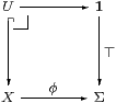
In our calculus, we shall use the λ-term φ:ΣX instead of the subset U⊂ X. A similar diagram, using the closed point ⊥∈Σ instead of ⊤, classifies (or, as we shall say, co-classifies) the closed subspace, that, classically, is complementary to U. We follow topology rather than logic in retaining the bijection between open and closed subspaces, even though they are not actually complementary in the sense of constructive set theory. This is because it is not sets but topological spaces that we wish to capture.
Unions and intersections of open and closed subspaces make the topology ΣX, and in particular the object Σ, into distributive lattices — honest ones now, not consisting of codes as in Remark 1.8. We therefore have to axiomatise the exponential and the lattice structure.
Axiom 3.3
The category S of “spaces” has finite products and an object Σ
of which all exponentials ΣX exist.
Then the adjunction Σ(−)⊣Σ(−)
that relates Sop to S is to be monadic.
This categorical statement has an associated symbolic form, consisting of
Remark 3.4
The equations required in parts (b) and (c) can each be formulated
in two different ways:
an abstract one that states the underlying monadic idea in λ-notation,
and a lattice-theoretic one that takes advantage of the additional
“topological” structure of the calculus.
One of our many tasks in this paper (Section 10)
is to prove the equivalence of these formulations.
In (b), we shall find that P:ΣΣX is prime iff it is a lattice homomorphism:
| P⊤⇔⊤ P⊥⇔⊥ P(φ∧ψ)⇔ Pφ∧ Pψ and P(φ∨ψ)⇔ Pφ∨ Pψ, |
whilst for (c), the term E is of the form I·Σi iff
| E(φ∧ψ) = E(Eφ∧ Eψ) and E(φ∨ψ) = E(Eφ∨ Eψ). |
We call such a term E a nucleus, shamelessly appropriating this word from locale theory, in which a nucleus is a monotone endofunction j:L→ L of a frame such that id≤ j=j· j. A nucleus E in our sense must be Scott continuous, but need not be order-related to the identity, but the senses agree when E≥id and j is Scott continuous.
We discuss Σ-split subspaces in Section 7, and give the admissibility equation in Definition 12.8, which is where we first use it in this paper.
Remark 3.5
We have said that we are interested in the term model of the calculus.
Now, this is powerful enough to encode computations,
because domain theory can be developed in it (Section 12)
and programming languages such as Plotkin’s PCF can be interpreted
using standard techniques of denotational semantics [Plo77].
This means that we cannot hope to give an explicit description
of the term model: the best we can do is to indicate how
the topological features of ASD can be “compiled out”,
to yield programs in some recognisable programming language.
In Sections B 9–11, arbitrarily complicated combinations of Σ-split subspaces and exponentials are reduced to a single Σ-split subspace of a (still complicated) exponential. In this paper (Section 8) we shall reduce this even further, to a Σ-split subspace of ΣN, showing that this description is equivalent to giving an N-indexed basis for X. The terms also have a corresponding normalisation.
This leaves focus, the quantifiers, recursion etc. on Σℕ. The idea of focus is that it recovers a point of a space from its Scott-open prime filter of neighbourhoods, which can be characterised using either infinitary lattice theory (Section A 2) or the λ-calculus arising from the monad (Section A 4) In this calculus, focus is pushed to the outside of any term, and is shown to be redundant at all objects except ℕ (Section A 8).
Using the (abstract) lattice structure and primitive recursion, focus on ℕ is inter-definable with definition by description (Section A 9). General recursion can also be defined. Finally, Section A 11 sketches how everything apart from disjunction and recursion strongly normalises, to what is essentially a Prolog clause. Restoring those two features yields a (parallel) Prolog program. On the other hand, normalising the λ-applications may not be such a good idea, so it’s better to think of ASD terms as parallel λ-Prolog programs.
The free model of the calculus therefore satisfies the Church–Turing thesis (i.e. it is equivalent to thousands of other ways of writing programs) so we do not need to introduce Kleene-style notation with Gödel numbers in order to justify calling it a computable account of topology. In particular, the “computations” referred to in Definitions 1.5, 1.6 and 2.3 may be defined by terms of our calculus.
Axiom 3.6
Returning to the Sierpiński space itself,
(Σ,⊤,⊥,∧,∨)
is an internal distributive lattice in S,
which also satisfies the Phoa principle,
| F:ΣΣ, σ:Σ ⊢ Fσ ⇔ F⊥ ∨ σ ∧ F⊤. |
This equation (which is bracketable either way, by distributivity) is used to ensure that terms of type ΣX yield data for the open or closed subspace of X, as required by the monadic axiom (Section C 3), and hence the pullback in Remark 3.2. It thereby enforces the bijective correspondences amongst open and closed subspaces and terms of type ΣX. We shall assert an “infinitary” generalisation of the Phoa principle shortly.
Definition 3.7
The lattice structure on Σ and ΣX defines
an intrinsic order, ≤, where
φ≤ψ iff φ=φ∧ψ iff φ∨ψ=ψ.
In the case of terms of type Σ (which we call propositions),
we shall write ⇒ and ⇔ instead of ≤ and =.
The order is inherited by other objects:
| Γ ⊢ a≤ b:X if Γ ⊢ (λφ:ΣX.φ a) ≤ (λφ.φ b):ΣΣX. |
There are other ways of defining an order, but sobriety and the Phoa principle make them equivalent, and also say that all maps are monotone (Section C 5).
In LKLoc this order on hom-sets arises from the order on the objects, considered as lattices, whilst in LKSp it is the specialisation order,
| x ≤ y ≡ (∀ U⊂ X open.x∈ U⇒ y∈ U) ≡ x ∈ |
| , |
where {y} is the smallest closed subspace containing y.

be the open and closed subspaces (co)classified by φ:ΣX. Then, with respect to the intrinsic orders on Σ and ΣX, there are adjoints
| ∃i⊣Σi and Σj⊣∀j |
that behave like quantifiers (Section C 3). (Note the different tails on the arrows.) ▫
Remark 3.9
The order ≤ on ΣX presents an important problem
for the axiomatisation of the join in Definition 3,
| φ = ⋁↑{β ∣ β≪φ}. |
The condition on the right of the “|” is monotone (covariant) in φ (indeed, Example 5.12 will use the fact that it is Scott-continuous), but contravariant with respect to β:
| if (β′≤β) then ((β′≪φ)⇐(β≪φ)). |
We want to regard the topology ΣX as another space, but the subset {β ∣ β≪φ} is not a sober subspace (in the Scott topology), since it isn’t closed under ⋁↑.
Remark 3.10
This means that we have, after all, to make a distinction between the
exponential space ΣX and the set (albeit structured)
of open subspaces of X. We shall write |ΣX| for the
latter, since it is the set of points of the space ΣX.
As there are â priori no “sets” in ASD, we have to explain
what special (properties of) spaces play their role in the theory.
As we shall see, one of these properties is an “equality test”.
Although locale theory plays down the underlying set functor |−|:Loc→Set, since it is not faithful, this functor nevertheless exists, and the subject makes intensive use of |ΣX| in particular, this being the frame corresponding to the locale X. The functor |−| may be characterised as the right adjoint to the inclusion Set→Loc that equips any set with its discrete topology, i.e. the powerset considered as a frame. In fact, this right adjoint is precisely what we have to add to the computably motivated axioms of abstract Stone duality given in this paper, in order to make them agree with the “official” theory of locally compact locales over an elementary topos [H] (which writes Ω X or UΣX for |ΣX|). In other words, it distinguishes between the two leading models in Remark 3.1.
This adjunction says that there is a map ε:|ΣX|→ΣX that is couniversal amongst maps β:N→ΣX from the objects N of a certain full subcategory, so β factors uniquely as N→|ΣX|→ΣX. However, the couniversal object |ΣX| cannot exist in the computable theory: besides being uncountable, its equality test would solve the Halting Problem. So we have to develop alternatives to it. In traditional language, all we need is that any φ∈ΣX be expressible as a directed join of βns, as in Definition 2.3.
Returning to the problem of Definition 3, we must use codes for (basic) open sets, since we cannot define ≪ in abstract Stone duality using the open set β:ΣX itself. Thus Remark 6.13 will replace the formula β≪φ (with variables β and φ) by
| n:N, φ:ΣX ⊢ (βn≪φ):Σ, |
where βn is the basic open subspace with code n.