


In this section we shall prove Dedekind’s main result, that any cut of R corresponds to an element of R, and not one of a yet more complicated structure. However, in order to say what a “Dedekind cut of R” is, we must finish the proof that its order (Definition 6.10) is dense without endpoints, i.e. that it satisfies Definition 6.1. This in turn requires that the object R be overt and Hausdorff.
In this section we shall be particularly careful to state the inclusion j:Q→ R that we defined in Lemma 6.12 by q↦(δq,υq), although we usually elide it elsewhere.
Lemma 9.1
Any property Φ that is true of some real number
(i.e. a cut a≡(δ,υ)),
is also true of some interval [e,t] around it,
in the sense that
|
So in particular it is true of any sufficiently close rational e or t, i.e.
| Φ(i x) ≡ Φ(δ,υ) =⇒ ∃ q:Q.Φ(δq,υq) ≡ ∃ q:Q.Φ(i j q). |
Note, however, that we cannot yet write ∀ x:[e,t].Φ(i x), but see Corollary 10.8.
Proof The first part is Proposition 7.12 in the case where (δ,υ) is a cut (rounded, bounded, disjoint and located). For the second part, δe⊑δt and υt⊑υe. ▫
Theorem 9.2 R is overt,
in which the existential quantifier satisfies the rule
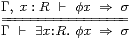
|
for any Γ⊢φ:ΣX, σ:Σ, where
| ∃ x:R.Φ(i x) ⇔ ∃ q:Q. Φ(i j q) ⇔ E1Φ(⊤,⊤) ⇔ EΦ(⊤,⊤) ⇒ Φ(⊤,⊤). |
However, the converse of the last implication fails for Φ≡∇ (Lemma 7.5).
Proof This is an application of Lemma 5.13, using the fact that ΣQ×ΣQ is a lattice and IR is the subspace of it that is defined by the nucleus E1, which preserves ⊥.
Let’s also give the proof directly. As Q is overt, we already have the rule with Q in place of R. The top line (for R) entails the similar judgement for Q by restriction, and then this entails the common bottom line. Conversely, by Lemma 9.1, φ x ⇒ ∃ q:Q.φ(j q) ⇒ σ. Using it again,
| ∃ q:Q.Φ(δq,υq) ⇔ ∃ d< q< u.Φ(δd,υu) ⇔ ∃ d< u.Φ(δd,υu) ≡ E1Φ(⊤,⊤) |
by Proposition 7.12.
Finally, we can use Lemma 8.10 to interchange E and E1 in the definition of ∃, that is, EΦ(⊤,⊤)⇔E1Φ(⊤,⊤), because (⊤,⊤) is located. ▫
Next we consider the application to R of the axioms that we introduced for Q in Section 6, namely dense linear orders, roundedness, boundedness, disjointness and locatedness. Their definitions involve existential quantification over R, but by Theorem 9.2 we may replace this by quantification over Q.
Theorem 9.3
R is Hausdorff (Definition 4.12),
and < (Definition 6.10)
is a dense linear order without endpoints (Definition 6.1).
Proof By Proposition 6.14, if a≡(δ,υ) and b≡(є,τ) are cuts then
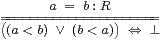
|
so R is Hausdorff, and the order satisfies the trichotomy law (Definition 6.1(c)); this is transitive by Lemma 6.11. It is extrapolative and interpolative in the sense that
| ⊤ ⇔ ∃ d u:Q.δ d∧υ u ⇔ ∃ d u.(δd,υd)<(δ,υ)<(δu,υu) |
and
| (δ,υ)<(є,τ) =⇒ ∃ q:Q.(δ,υ)<(δq,υq)<(є,τ), |
but this existential quantification over Q may be considered as one over R. ▫
We can now define Dedekind cuts over R, i.e. to formulate Definition 6.8 and essentially to repeat the construction with R in place of Q. In doing so, we find once again that the ascending and descending reals are natural intermediate steps. As before, it is easy to define them, and to show that they are the same, whether we start from Q or from R, cf. Exercise 2.2. After that, we simply have to show that the other conditions carve out R⊂R×R in the same way in both versions.
Proposition 9.4 The maps ΣQ⇄ΣR given by
| δ ↦ λ r:R.∃ e:Q.r< j e∧δ e and λ d:Q.Δ(j d) ↤ Δ |
restrict to a bijection between rounded lower δ:ΣQ and Δ:ΣR. Hence the two constructions of R agree. Those for R do so too, with
| υ ↦ λ r:R.∃ t:Q.j t< r∧υ t and λ u:Q.Υ(j u) ↤ Υ. |
Proof Recall from Lemmas 6.12f that j d<R j e⇔ d<Q e and (δ,υ)<R j u⇔υ u. Then
| Δ ↦ δ ↦ λ r.∃ e:Q.r< j e∧ Δ(j e) = λ r.∃ s:R.r< s∧ Δ(s) ≡ |
|
by Theorem 9.2, and δ ↦ Δ ↦ λ d.∃ e.j d<R j e∧δ e ≡ λ d.∃ e.d<Q e∧δ e ≡ δ. ▫
Proposition 9.5 Under this correspondence,
the rounded pseudo-cut (Δ,Υ) of R is respectively
disjoint, bounded or located iff the
pseudo-cut (δ,υ) of Q has the same property.
Proof For disjointness, using Theorem 9.2,
|
and the argument for B and boundedness just omits s< r and u< d.
If (δ,υ) is located then so is (Δ,Υ), because, since j d<R j t⇔ e<Q t⇒δ e∨δ t,
| r< s ⇒ ∃ e t:Q.r< j e< j t< s ⇒ (∃ e.r< j e∧ δ e)∨(∃ t.j t< s∧ υ t) ≡ Δ r∨Υ s. |
Conversely, if (Δ,Υ) is located then so is (δ,υ), because
| d<Q u ⇔ j d<R j u ⇒ Δ(j d)∨Υ(j u) ≡ δ d∨υ u. ▫ |
Theorem 9.6
(R,<) is a Dedekind-complete
dense linear order without endpoints,
in the sense that every cut (Δ,Υ):ΣR×ΣR
(possibly involving parameters) is of the form
| Δ = λ x.(x< a) and Υ = λ y.(a< y) |
for some unique a:R (with the same parameters).
Proof The real number a is the cut (δ,υ) of Q given by the above correspondence. It satisfies
| x < a < y ⇔ (∃ e:Q. x< j e∧δ e)∧(∃ t:Q.j t< y∧υ t) ≡ Δ x∧ Υ y. ▫ |
Remark 9.7
In the previous section, the construction of R from Q
involved the formulation of the nucleus E.
However, we cannot repeat this step with R in place of Q,
because existential quantification over finite lists in R is not allowed
in Notation 8.2.
Why on Earth not? This has nothing to do with rational or irrational numbers: so far the elements of Q are only nominally “rational”, as we have not introduced any arithmetic yet. The point is topological: Q is overt discrete — essentially a “set” — and List (Q) is the overt discrete “hyperspace” of its overt compact subspaces (Theorem 5.21). On the other hand, R is not discrete but Hausdorff, and its overt compact subspaces can be infinite — bounded closed intervals, for example. In the hyperspace of such subspaces, the finite ones form a dense subspace, so there is no way to distinguish them from the infinite ones.
But this does not matter. We do not need to define another space S↣ΣR×ΣR from such an E, as we have already done enough to prove completeness, so R itself serves for S. Then
| R ↣ IR↣ |
| × |
| ↣ΣR×ΣR |
is a composite of Σ-split inclusions. In fact, the splitting will be expressible in the same way as in Proposition 2.15, after we have proved compactness of [d,u] (Proposition 14.7).
Two other important notions of completeness for the real line are considered in [J], namely the convergence of Cauchy sequences (Theorem J 6.14) and the existence of suprema of nonempty bounded subsets (Theorem J 12.9). In any form of constructive analysis, the latter result requires additional hypotheses; in ASD these are that the subset be compact and overt.
A natural special case of the supremum is the maximum of a pair:
Proposition 9.8
R has binary join and meet with respect to ≤,
|
satisfying min(a,b)≤ a,b≤max(a,b) and
| ▫ |
We have said that the two halves of a Dedekind cut play symmetrical roles. Adding an operation that makes this literally so, we have the beginnings of arithmetic:
Proposition 9.9
If (Q,<) has an order-reversing automorphism (−)
then so does R, and this has a unique fixed point (0):
| ⊖(δ,υ) ≡ (λ d.υ(−d), λ u.δ(−u)) 0 ≡ (λ d.d< −d, λ u.−u< u). |
This agrees with Moore’s interval arithmetic, since ⊖(δd,υu)=(δ−u,υ−d). Since it preserves roundedness, it defines an isomorphism R≅R (Definition 7.3), but not an automorphism of either of them. Since it also preserves disjointness, boundedness and locatedness, we have ⊖:IR≅ IR and −:R≅ R.
From negation and maximum we may define the absolute value function,
| |(δ,υ)| ≡ max((δ,υ), −(δ,υ)) = (λ d.δ d∨υ(−d), λ u.υ u∧δ(−u)), |
so |x| = x if x≥ 0 and |x| = −x if x≤ 0.
This satisfies
(x≠0)≡(δ 0∨υ 0)⇔|x|≠ 0.
▫
We shall develop addition and multiplication in Sections 11 and 12, and we use Dedekind completeness to find the inverses of strictly monotone functions in Section 13, but now we turn to the Heine–Borel theorem.