


We have seen how some of the ideas of topology can be expressed using the types and terms of a λ-calculus. In particular, compactness of a space K is expressed as a “universal quantifier” ∀K:ΣK→Σ. The main application of this idea will be to the closed interval K≡[d,u]⊂ R⊂Σℚ×Σℚ≡ Y, where we shall construct R as the subspace of those pairs of predicates on ℚ that are Dedekind cuts (Remark 2.1).
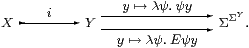
How could we obtain a map ΣK→Σ from one i:K↣ Y? We have ΣY→Σ by evaluation at some y:Y (Lemma 5.12), but nothing ΣK→ΣY, since the maps go the wrong way. However, given that we have already introduced higher types, it hardly seems to be a revolutionary step to introduce extra terms of those types. Indeed, in our brief account of interval analysis in Section 2, we have already discussed such a map, I:ΣK→ΣY. It extends open sets and functions from the real line to the interval domain, and it is intimately related to the quantifiers ∀ and ∃, indeed these are special cases of it.
In this section we shall give the type-theoretic rules that formally introduce i and I for (certain) subspaces, at least the ones that we need. This will complete our manual of the axioms of ASD. The basis of our proof of the Heine–Borel theorem is that the rules force these subspaces to carry the subspace topology. Naturally, we shall use terms of higher type (such as I) to do this, just as we have already introduced terms of lower type and equations between them in the previous section.
Definition 5.1 An inclusion i:X↣ Y
is called a Σ-split subspace
if there is another map I:ΣX↣ΣY such that
| Σi· I = idΣX or x:X, φ:ΣX ⊢ Iφ(i x) ⇔ φ x, |
thereby making ΣX a retract of ΣY with inclusion I and projection Σi. The convention in the λ-calculus is that Iφ(i x) means (Iφ)(i x).
Remark 5.2 Whenever two maps compose to the identity one way round like this,
they may be recovered (uniquely up to unique isomorphism) from their
composite the other way, which is an idempotent (E=E· E).
In this case, E≡ I·Σi:ΣY→ΣY
determines ΣX.
(We wrote E for E in Proposition 2.15 in accordance
with our convention of using fancier typefaces for fancier types.)
The object X itself is the equaliser
The idea is that the operator E “normalises” open subspaces of Y by restricting them to X using Σi, and then re-expanding them using I. Therefore a:Y belongs to {Y ∣ E} iff its membership of any open subspace ψ of Y is unaffected by this process.
Definition 5.3 Recall that being the equaliser means that
Not every idempotent E on ΣY can arise in this way from a Σ-split subspace, because the surjective part Σi of its splitting must be a homomorphism for the topological structure. In particular, it must preserve the four lattice connectives, but any order-preserving surjective function between lattices preserves ⊤ and ⊥ anyway. So the crucial condition is this:
Lemma 5.4
E≡ I·Σi:ΣY→ΣY satisfies the equations,
for φ,ψ:ΣY,
| E(φ∧ψ) = E(Eφ∧ Eψ) and E(φ∨ψ) = E(Eφ∨ Eψ). ▫ |
Definition 5.5 A term E
that satisfies the equations in the Lemma is called a nucleus.
In order to avoid developing a theory of dependent types,
we do not allow E to have parameters.
The word “nucleus” was appropriated from locale theory, since both kinds of nuclei play the same role, namely to define subspaces, but the definitions are different. A localic nucleus, usually called j, must satisfy id⊑ j=j· j but need not be Scott-continuous [Joh82, §II 2]. Nuclei in ASD, on the other hand, are continuous but need not be order-related to id. So the common ground is when E⊒id and j is continuous: ASD and locale theory therefore agree on how to form closed subspaces, but not open ones or retracts.
In Section 8 we shall use E to define R as a subspace of the interval domain IR, and in this case E is a nucleus in both senses. If we view R instead as a subspace of Σℚ×Σℚ, but still defined by E, this is a nucleus only in the sense of ASD, not that of locale theory.
Notation 5.6 We write {Y ∣ E} for the subspace X⊂ Y
that is defined by any nucleus E on Y.
Beware, however, that this has very few of the properties of
subset-formation in set theory.
Definition 5.7
A term a:Y (which may now involve parameters from a context Γ)
of the larger space Y is called admissible with respect to
the nucleus E if
| Γ, ψ:ΣY ⊢ ψ a ⇔ Eψ a. |
This is the same as saying that the map a:Γ→ Y has equal composites with the parallel pair in the diagram in Remark 5.2, so it factors through the equaliser.
Since this equaliser is the subtype X⊂ Y, we may then regard a as a term of type X or {Y ∣ E}. However, when we need to discuss the calculus in a formal way, we shall write admitY,E a for it, in order to disambiguate its type.
Remark 5.8
The simplest (and first,
Section C 3)
application of this
calculus is to the construction of open and closed subspaces.
This will formalise Remark 4.11.
Let θ:ΣY be a closed term (i.e. without parameters), which we think of as a continuous function θ:Y→Σ. The open and closed subspaces that θ (co)classifies are the inverse images U≡θ−1(⊤) and C≡θ−1(⊥) of the two points of the Sierpiński space (Remark 3.2).
Classically, any open subspace of U is already one of Y, whilst an open subspace of C becomes open in Y when we add U to it. This means that
| ΣU ≅ ΣY↓θ ≡ {ψ ∣ ψ⊑θ} and ΣC ≅ θ↓ΣY ≡ {ψ ∣ ψ⊒θ}, |
i.e. the parts of the lattice ΣY that lie respectively below and above θ. (The ↓ notation is used in category theory for “slice” or “comma” categories.)
From this we see what the Σ-splittings and nuclei for U and C must be. The construction of the interval domain IR⊂Σℚ×Σℚ in Section 7 will involve an open subspace, a closed one and a retract.
Lemma 5.9
Let e:Y→ Y be an idempotent and θ:Y→Σ any map. Then
| Σe, θ∧(−) and θ∨(−) |
are nuclei on Y, with respect to which a:Y is admissible iff respectively
| e a=a, θ a⇔⊤ and θ a⇔⊥. ▫ |
Notation 5.10 As we shall need to name the Σ-splittings
of j:U,C↣ Y, we write
| ∃j:ΣU↣ΣY and ∀j:ΣC↣ΣY, |
where ∃j(Σjψ)=ψ∧θ and ∀j(Σjψ)=ψ∨θ. See [C] for the reasons for these names.
In Sections 7 and 8 we shall need to combine several nuclei. However, the intersection of two Σ-split subspaces need not exist, in general, and even if it does, it need not be Σ-split. Everything works if the nuclei commute, but this does not often happen. In fact, there are many situations in which E1· E2· E1=E1· E2, and that is sufficient to justify forming the intersection.
Lemma 5.11 Let E1 and E2 be nuclei on a type Y
such that either E1· E2=E2· E1 or
E1· E2· E1=E1· E2.
Then E1· E2 is also a nucleus, and defines the intersection (pullback)
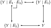
in which all five inclusions (including the composite) are Σ-split. Regarding {Y ∣ E1}⊂ Y as the subset of admissible elements, and Σ{Y ∣ E1} as the subset {ψ:ΣY ∣ E1ψ=ψ}, we see E1· E2 as a nucleus on {Y ∣ E1} but not necessarily on {Y ∣ E2}. ▫
We have already said that nuclei and Σ-splittings are intimately related to the quantifiers that define compactness and overtness. The following two lemmas will provide the key to defining ∃ and ∀ from I in Section 10. There we shall use the slices Σℚ×Σℚ↓(δu,υd) and (δd,υu)↓Σℚ×Σℚ, which we shall call lattices in this very specific context.
Lemma 5.12 Any lattice L is overt and compact, with
∃Φ≡Φ(⊤) and ∀Φ≡Φ(⊥).
Proof By monotonicity, Φ(⊥)⇒Φ(x)⇒Φ(⊤) for any x:L. ▫
Lemma 5.13
Let i:X↣ L and I:ΣX↣ΣL with
Σi· I=id. Then2
Proof In each column we deduce in both directions,
|
using Axiom 4.7 and Definition 4.14. ▫
It is high time we gave the actual rules that define subtypes and their admissible terms. These formally adjoin Σ-split subspaces to the calculus just as number theorists formally adjoin roots of particular polynomials to a field, or set theorists construct “equiconsistent” models that have altered properties. Theorem 15.8 describes the corresponding categorical construction.
As in type theory, we name the rules after the connective that they introduce or eliminate. Our connectives are called {} and Σ{}.
Axiom 5.14
The {}-rules of the monadic λ-calculus
define the subspace itself:
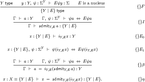
These rules say that {Y ∣ E} is the equaliser in Remark 5.2.
Axiom 5.15
The following Σ{}-rules say that
{Y ∣ E} has the subspace topology,
where IY,E expands open subsets of the subspace to the whole space.
| φ:Σ{Y ∣ E} ⊢ IY,Eφ:ΣY. Σ |
| E |
The Σ{}I rule is derived from {}E0:
| ψ:ΣY ⊢ Σiψ ≡ λ x:{Y ∣ E}.ψ(iY,E x):Σ{Y ∣ E}. Σ |
| I |
The β-rule says that the composite Σi;I:ΣY↠Σ{Y ∣ E}↣ΣY is E:
| y:Y, ψ:ΣY ⊢ IY,E(λ x:{Y ∣ E}.ψ(iY,E x))y ⇔ Eψ y. Σ |
| β |
The η-rule says that the other composite Σ↣↠ΣY↠Σ{Y ∣ E} is the identity:
| φ:Σ{Y ∣ E}, x:{Y ∣ E} ⊢ φ x ⇔ IY,Eφ(iY,E x). Σ |
| η |
This equation is the one in Definition 5.1 for a Σ-split subspace.
Remark 5.16 Notice that the Σ{}β-rule
is the only one that introduces E into terms.
This is something that we want to avoid if at all possible,
given that the expressions for nuclei, such as E,
which we intend to use to construct R, are usually very complicated.
The normalisation theorem that eliminates unnecessary Es is proved
in Section B 9–10.
When E does find its way into a program, it will give rise to a substantial computation. But this is what we would expect, considering the relationship to the quantifiers, and their computational meaning as optimisation and search (Section 2).
Warning 5.17
It is important to understand that,
for another structure to admit a valid interpretation of this calculus,
not only must the equaliser in Remark 5.2 exist,
but there must also be a map I in the structure that satisfies
the equations Σi· I=idΣX and I·Σi=E,
cf. Remark 2.18.
|
Remark 5.19 If this paper is the first one about ASD that you have seen,
you may reasonably imagine that we have cooked up the rules
from the observations in Section 2,
based on little more than the properties of the real line
that first year undergraduates learn.
Can this theory of topology even be generalised to ℝn?
Is it of any use in proving theorems in mathematics other than those
that we have mentioned?
Actually, we have told the story so far in reverse historical order. The calculus above was derived from a categorical intuition, and when it was formulated [B], it was a solution in search of a problem. There were no clear ideas of how the real line might be constructed, and certainly no inkling that it might behave in ASD in a radically different way from the established theory of Recursive Analysis (Section 15). That it turned out to do so is a tribute to category theory as a source of, or rather as a way of communicating, mathematical intuitions.
For reference we give a summary of some of the constructions that have been performed using nuclei in the infrastructure of ASD.
Theorem 5.20 Σ-split subspaces interact with the underlying
structure of products and exponentials as follows,
and also provide stable disjoint unions
Section B 11.
|
In Section 8, we shall need to perform some combinatorial arguments using lists of rational numbers. However, since ASD is a direct axiomatisation of topology, without using set theory, we have to recover some kind of “naïve set theory” within our category of spaces. Our “sets” are the overt discrete objects.
Theorem 5.21
The full subcategory consisting of the overt discrete objects has
This categorical structure is called an arithmetic universe. ▫
Remark 5.22
We shall rely on this result to provide the “discrete mathematics”
that we need, namely
The infinite objects that are generated in this way are countable in the strict sense of being bijective with a decidable subset of ℕ in the calculus; since our isomorphisms are homeomorphisms, such objects inherit =, ∃, and in some cases ≠, from ℕ.
These “sets” do not admit a full powerset on the basis of the axioms that we have given here, and therefore they do not form an elementary topos or model of set theory. However, it is possible to add another (much more powerful, and certainly non-computational) axiom to ASD that does make the full subcategory of overt discrete objects into a topos. This axiom asserts that this subcategory is co-reflective, i.e. that the inclusion has a right adjoint, which formally assigns an overt discrete object to any space, and we call this object the “underlying set” of the space [H]. We do not use this axiom in this paper.
Remark 5.23
In order to formulate the definition of Σ-split subspace
we only need powers Σ(−),
not the lattice structure on Σ or the quantifiers.
The category-theoretic summary of this section is that we require
the adjunction Σ(−)⊣Σ(−) to be monadic.
The notions of sobriety and Σ-split subspaces in ASD come from the two conditions in the theorem of Jon Beck (1966) that characterise monadic adjunctions [Tay99, Theorem 7.5.9]. Sobriety says that Σ(−) reflects invertibility (Proposition 4.23). Nuclei are essentially the same as Σ(−)-contractible equalisers; Axiom 5.14 says that such equalisers exist, and Axiom 5.15 that Σ(−) takes them to coequalisers. These conditions are given as equations between higher-order λ-terms in [A][B].
In the presence of the other topological structure in the previous section, in particular Scott continuity, the equations that define a nucleus are equivalent to the much simpler ones involving finitary ∧ and ∨ that we gave in Lemma 5.4 and Definition 4.22 [Section G 10]. In this setting, any definable object X of ASD can be expressed as a Σ-split subspace, i:X↣Σℕ, where i and I correspond directly to a basis of open subspaces and related compact subspaces. Locally compact spaces and computably continuous functions between them can then be understood directly in ASD [G]. This calculus is how we implement the foundations of recursive analysis and topology based on open sets instead of points.
However, the introduction of nuclei with this definition after the lattice theory in the previous section is the reason why our discussion of open and closed subspaces and the Phoa principle in Remark 4.11 was deductively unsatisfactory. From a foundational point of view, the monadic structure should really come first. Then the Euclidean principle (σ∧ Fσ⇔σ∧ F⊤), which is the part of the Phoa principle that applies to intuitionistic set theory or the subobject classifier in an elementary topos, is exactly what is required to make Eφ≡φ∧θ a nucleus in the abstract sense, or equivalently to justify the first of the two Gentzen-style rules. This is essentially how this principle was discovered [Section C 3].
The results that we have sketched here are treated in greater detail in the earlier papers that developed ASD. The foundations of the theory, together with the methodology and motivations behind it, are surveyed in [O].