4  The ASD lambda calculus

This section and the next summarise the symbolic language for ASD in a “user manual” style. Beware, however, that the manual for some device does not make its engineering redundant, and indeed the development of the more powerful devices of the future depends on advances in the underlying principles. Nevertheless, the constructions in the rest of this paper will be made entirely within this calculus. We repeat that there is no underlying set theory, and that the monadic and Phoa principles are unalienable parts of the system. On the other hand, there are other formulations of Scott continuity of various strengths besides the one that we give here.

Axiom 4.1 The types of ASD are generated from

1. base types 1, Σ and ℕ, by
2. products, X× Y,
3. exponentials, Σ^X, or X→Σ if you prefer, and
4. Σ-split subspaces.

We do not introduce general exponentials Y^X, infinitary products, type variables or dependent types — at least, not in this version of the calculus. We will explain Σ-split subspaces, which abstract Proposition 2.15, in the next section; they will be used to define open, closed and retract subspaces, and, of course, R itself.

Axiom 4.2 The logical terms of type Σ or Σ^U (also known as propositions and predicates respectively) are generated from

1. constants ⊤ and ⊥;
2. the lattice connectives ∧ and ∨ (but not ⇒ or ¬);
3. λ-abstraction λ x.φ, where φ must itself be logical (i.e. of some type of the form Σ^V, and in particular not ℕ or ℝ), but x may be of any type;
4. λ-application φ a, where a:A, and φ:Σ^A is logical;
5. equality (n=_N m), where N is any discrete type;
6. inequality or apartness (h≠_H k), where H is any Hausdorff type;
7. existential quantification ∃ x:X.φ x, where φ x is logical, and the type X is overt;
8. universal quantification ∀ k:K.φ k, where φ k is logical, and the type K is compact.

These terms are generated within a larger calculus that also includes

1. variables of all types, for which we use increasingly exotic alphabets as the types get more complex; and
2. pairing < , > and projections π₀, π₁ for product types.

Discrete, Hausdorff, overt and compact spaces will be defined shortly. Existential quantification over ℕ or ℝ is allowed, but universal quantification is not. Universal quantification over the closed interval I≡[0,1] is justified in Section 10.

So examples of invalid logical formulae include

but (∃ n p q r:ℕ.pⁿ+qⁿ=rⁿ) and (∀ x:|x|≤ 2.x²< 0) are fine. Programs to which an Ml compiler would assign the types nat→nat or real→real are treated in ASD as terms of type ℕ→ℕ_⊥ or ℝ→ℝ_⊥ [D][F].

Binding, renaming, duplication, omission and substitution for variables are the same as in the λ- and predicate calculi. A quantified formula has the same type as its body (φ), whilst λ-abstraction and application modify types in the usual way. Alternating quantifiers are allowed to any depth — so long as their ranges are overt or compact spaces.

Axiom 4.3 The numerical terms of type ℕ are generated from

1. the constant 0;
2. variables;
3. successor; and
4. definition by description: the  n.φ n (Axiom 4.24).
5. We also allow primitive recursion over ℕ at any type X.

Definition 4.4 Judgements in the calculus are of the four forms

asserting well-formedness of types and typed terms, and equality or implication of terms. We shall refer to a=b and α⊑β on the right of the ⊢ as statements. On the left is the context Γ, consisting of assignments of types to variables, and maybe also equational hypotheses  (Section E 2).

The form Γ ⊢ α⊑β:Σ^X is syntactic sugar:

Axiom 4.5 The predicates and terms satisfy certain equational axioms, including

1. those for a distributive lattice; in particular, for Γ⊢φ,ψ:Σ^X we write

   φ  ⊑  ψ   to mean   φ∧ψ  =  φ,   or equivalently   φ∨ψ  =  ψ,

   although for σ,τ:Σ we use σ⇒τ and σ⇔τ instead of σ⊑τ and σ=τ, since we shall also need the symbols ≤ and = for their more usual “numerical” meanings;
2. the β- and η-rules for λ-abstraction/application and pairing/projection;
3. the β- and η-rules for primitive recursion over ℕ; and
4. others that we describe in a little more detail in the rest of this section.

Remark 4.6 Predicates and terms on their own denote open subspaces and continuous functions respectively, but their expressive power is very weak. We introduce implications into the logic, but make their hierarchy explicit, in the form of statements and judgements.

1. Observe, first, that ⊑, =, ⇒ and ⇔ link predicates to form statements, not new predicates. In other words, Σ is a lattice and not a Heyting algebra.
2. There are equality statements a=b:X for any type, but equality predicates (n=_N m):Σ only for discrete types. In particular, for a,b:R, there are predicates a≠ b and a< b, but a=b and a≤ b are statements, since R is Hausdorff but not discrete.
3. For any proposition σ, we sometimes write σ or ¬σ for the statements σ⇔⊤ or σ⇔⊥.
4. Nested equality and implication are not allowed in statements: we use a judgement of the form α₂⇒β₁⊢γ₁⇒δ₀ instead. If we need another level of nesting, we use a proof rule: See Exercise 6.17 for some examples. This is as far as we can go. This rather artificial limit will be rectified in a future extended calculus [M].
5. Equality and implication statements for function-types Σ^X provide a way of stating quantification over any type X — as a statement — it’s a predicate only when X is compact. However, for the sake of clarity, we usually write Γ,x:X⊢φ x⇔ψ x instead of Γ⊢φ=ψ.

Our convention is that λ-application binds most tightly, followed by the propositional relations, then ∧, then ∨, then λ, ∃ and ∀, then ⇒, ⇔, ⊑, = and finally ⊢. This reflects the hierarchy of propositions, predicates, statements, judgements and rules. We often bracket propositional equality for emphasis and clarity.

Axiom 4.7 In addition to the equations for a distributive lattice, Σ satisfies the rules¹

Axiom 4.8 Every F:Σ^Σ is monotone, i.e. F⊥⇒ F⊤.

Lemma 4.9 Σ satisfies the Phoa principle, Fσ  ⇔ F⊥ ∨ σ∧ F⊤, for F:Σ→Σ and σ:Σ, possibly involving parameters.         ▫

Plainly Phoa entails monotonicity, and we shall explain shortly why the Gentzen-style rules in Axiom 4.7 are also derivable from it.

Definition 4.10 We say that φ:Σ^X classifies an open subspace of X, and co-classifies a closed one. In symbols, for a:X,

so U⊂ U′ iff C′⊂ C iff φ⊑φ′. This means that

are in bijection. A clopen, complemented or decidable subspace is one that is both open and closed. Then it and its complement are the inverse images of 0,1∈2 under some (unique) map X→2 Theorem B 11.8 [Proposition C 9.6].

Remark 4.11 Such inverse image types cannot of course be generated from ℕ and Σ by × and Σ⁽⁻⁾. Our comments here will be justified by the introduction of open and closed subspaces as Σ-split subspaces in the next section. Briefly, being Σ-split means that all open subsubspaces of a subspace are restrictions of open subspaces of the ambient space, indeed in a canonical way.

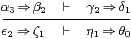
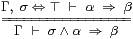
Consider the left-hand Gentzen rule in terms of the open subspaces that α, β and σ classify. The top line expresses the containment α⇒β of open subsubspaces of the open subspace classified by σ. In the ambient space, this means that α∧σ⇒β∧σ, or, more briefly, α∧σ⇒β, as in the bottom line.

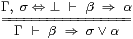
The rule on the right says exactly the same thing, but for the intersection of closed subspaces. Translating this into a result about relatively open subsubspaces of the closed subspace, the relative containment β⇒α in the closed subspace means β∨σ⇒α∨σ, or just β⇒α∨σ, in the whole space.

Another “extensional” aspect of topology that the rules state is that, if the inverse images of ⊤ under φ,ψ:X⇉Σ coincide as (open) subspaces of X, then x:X⊢φ x⇔ψ x (or φ=ψ) as logical terms. The inverse images of ⊥ behave in a similar way [Section C 5].

Subspaces of X² or X³ are often called binary or ternary relations. In particular, open binary relations are the same thing as predicates with two variables.

Definition 4.12 If the diagonal subspace, X⊂ X× X, is open or closed then we call X discrete or Hausdorff respectively. Type-theoretically, such spaces are those in which we may internalise equality-statements as predicates:

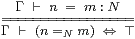
Lemma 4.13 Equality has the usual properties of substitution, reflexivity, symmetry and transitivity, whilst inequality or apartness obeys their lattice duals:

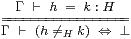
(The proof of this uses Axiom 4.7.) In an overt discrete space, or a compact Hausdorff one, we have the converse of the first of the four rules:

When both =_X and ≠_X are defined, as they are for ℕ, they are complementary:

In this case X is said to have decidable equality.         ▫

Definition 4.14 A space X that admits existential or universal quantification is called overt or compact respectively. By these quantifiers we mean the type-theoretic rules

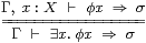
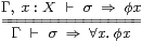
Axiom 4.15 The space ℕ is overt. This and Scott continuity break the de Morgan-style lattice duality that the other rules enjoy.

Remark 4.16 So long as the types of the variables really are overt or compact, we may reason with the quantifiers in the usual ways:

1. If we find a particular a:X that satisfies φ a, then we may of course assert ∃ x.φ x. This simple step tends to pass unnoticed in the middle of an argument, in the form φ a⇒∃ x.φ x.
2. Similarly, if the judgement ∀ x.φ x has been proved, and we have a particular value a:X, then we may deduce φ a. Again, we often just write (∀ x.φ x)⇒φ a.
3. The familiar mathematical idiom “there exists”, in which ∃ x.φ x is asserted and then x is temporarily used in the subsequent argument, is valid, as [Tay99, §1.6] explains.
4. The λ-calculus formulation automatically allows substitution under the quantifiers [Section C 8], whereas in categorical logic this property must be stated separately, and is known as the Beck–Chevalley condition [Tay99, Chapter IX].

However, we must observe the caveats in Remarks 3.5 and 15.4:

1. Given ∃ x.φ x, there need only be a term a:X satisfying φ a in the case where X and the types all of the parameters in φ are overt discrete and Hausdorff.
2. We cannot deduce ∀ x.φ x from proofs of φ a for every closed term a:X.

Exercise 4.17 Use the Phoa principle to prove the Frobenius and modal laws

where the type of x is both overt and compact. The Frobenius law for ∀ is another feature that ASD has in common with classical but not intuitionistic logic; it was nevertheless identified in intuitionistic locale theory by Japie Vermeulen [Ver94].         ▫

Lemma 4.18 Any topology Σ^X has joins indexed by overt objects and meets indexed by compact ones:

Binary meets distribute over joins by the Frobenius law, and “substitution under the quantifier” means that all inverse image maps Σ^f:Σ^Y→Σ^X , where

preserve all joins indexed by overt objects, and meets indexed by compact ones [Section C 7].         ▫

Since ℕ is overt but not compact, each Σ^X has and each Σ^f preserves ℕ-indexed joins, but not ℕ-indexed meets.

Remark 4.19 We often want the quantifiers or meets and joins to range over dependent types, even though we have not provided these in the calculus.

The most pressing case of this is the join or existential quantifier indexed by an open subspace M⊂ N of an overt space. This subspace is classified by a predicate α:Σ^N, which we shall write as Γ,  n:N ⊢ α_n:Σ. The M-indexed family φ^m:Σ^X of which we want to form the join may always be considered to be the restriction to M of an N-indexed family, so we have

This sub- and super-script notation, which is used extensively in [G], indicates co- and contra-variance with respect to an imposed order relation, such as the arithmetical order in ℚ or inclusion of lists.

We shall also want to define both quantifiers over the closed interval [d,u], where d and u need not be constants, but we shall cross this bridge when we come to it, in Section 10.

Definition 4.20 Such a pair of families (α_n,φⁿ) is called a directed diagram, and the corresponding

is called a directed join, if (a) (∃ n.α_n)⇔⊤, and (b) α_{n @ m}⇔α_n∧α_m and φ^{n @ m}⊒φⁿ∨φ^m for some binary operation @:N× N→ N.

In this, α_n∧α_m means that both φⁿ and φ^m contribute to the join, so for directedness in the informal sense, we require some φ^{n @ m} to be above them both (contravariance), and also to count towards the join, for which α_{n @ m} must be true (covariance). Hence the imposed order relation on N is that for which (N,@) is essentially a meet semilattice.

This allows us to formalise Scott continuity (Definitions 2.6 and 3.1).

Axiom 4.21 Any F:Σ^ΣX (possibly with parameters) preserves directed joins in the sense that

Notice that F is attached to φⁿ and not to α_n, since the join being considered is really that over the subset M≡{n ∣ α_n}⊂ N. The principal use of this axiom in this paper is Proposition 7.12, where the ambient overt object N is ℚ, and its imposed order is either the arithmetic one or its reverse, so @ is either max or min. Scott continuity is also what connects our definition of compactness with the traditional “finite open sub-cover” one (Remark 10.10), whilst in denotational semantics it gives a meaning to recursive programs.

In locale theory [Joh82], the homomorphisms are those of finite meets and arbitrary joins. Since we have just taken care of (some of) the directed joins, in ASD we need only consider the finitary connectives ⊤, ⊥, ∧ and ∨.

Definition 4.22 A term P of type Σ^ΣX is called prime if it preserves all four lattice connectives:

The type X is said to be sober if every prime P corresponds to a unique term a:X (which we call focusP) such that

Proposition 4.23 Let i:X→ Y between sober objects. If the map Σⁱ:Σ^Y→Σ^X has an inverse I, then so does i itself [Tay91].

Proof    The map η:Y↣Σ^ΣY given by y↦λψ.ψ y is mono, because focus_Y(λψ.ψ y)=y.

Since I is an isomorphism, both it and P≡λφ.Iφ y preserve all four lattice operations, i.e. P is prime. Then, as X is sober, we may define j:Y→ X by j y≡focus_X(λφ.Iφ y). It satisfies

so i(j y)=y since η:Y↣Σ^ΣY is mono.         ▫

For ℕ, sobriety is equivalent to a more familiar idiom of reasoning that characterises singleton predicates, φ={n}≡(λ m.n=m). This is only meaningful for (overt) discrete objects, but we shall see in Section 14 that Dedekind completeness expresses sobriety of ℝ.

Axiom 4.24 A predicate φ n for n:ℕ (possibly involving other parameters) is called a description if it is “uniquely satisfiable” in the sense that

are provable. Then we may introduce the  n.φ n:ℕ, with the same parameters, satisfying

Descriptions may be used to define general recursion (minimalisation) [A][D][O].

Proposition 4.25 All types that are definable from 1, Σ and ℕ using × and Σ⁽⁻⁾ are sober.

Proof    

1. The only prime of type Σ^Σ1 is P≡λφ.φ⋆, and focus₁P=⋆.
2. If P:Σ^Σℕ is prime then φ n≡ P(λ m.n=_ℕm) is a description, and focus_ℕP=the  n.φ n
   Section A 10.
3. If X and Y are sober then so is X× Y, with

   focusX× Y P  =  <focusX(λφ.P(λ p.φ(π0 p))), focusY(λψ.P(λ p.ψ(π1 p)))>.

4. Any Σ^X is sober, with focus_Σ^XP≡λ x.P(λφ.φ x) Lemma A 8.8.         ▫

Examples 4.26 We conclude with some examples of the four main topological properties.

The axioms only provide the quantifiers ∀_∅≡⊤, ∃_∅≡⊥, ∀₂≡∧, ∃₂≡∨ and ∃_ℕ directly — it is the business of this paper to construct ∃_ℝ, ∃_I and ∀_I, in Sections 9 and 10. To put this the other way round, assuming that a future extension of the calculus will allow arbitrary nesting of ⇒ and ∀ in statements (cf. Remark 4.6), these constructions will justify quantifier elimination in the corresponding cases.

The calculus as we have described it so far will be used to define individual Dedekind cuts in Section 6.