


In this section we add the lattice structure on Σ and either the Euclidean or the Phoa principle to the monadic framework that we introduced in §6. The latter plays (part of) the role of the set theory that we take granted when we study other subjects such as group theory, but which we have eschewed for computable topology. So the theory will start to look a little more like an “orthodox” development of theorems from axioms (§3.2).
See [C][D] for the details of the results in this section, but, despite the lettering, they were written before the monadic λ-calculus of §6 was devised, so it was expressed in a less clear categorical language. Since the empirical arguments were also not as well developed there as they were in the previous section, we shall give some of the basic results here in detail. On the other hand, [I][J] give better treatments of some topics that are closer to the applications, especially the theory of compact subspaces.
8.1.
In addition to the axioms in §6.1,
we now require the type Σ to have
where σ:Σ and F:ΣΣ.
8.2.
The lattice structure defines an order relation on Σ
and its powers ΣX.
Following logical custom,
we have already started to write ⇒ and ⇔
for the order and equality on Σ.
We retain ⊑ and = for these relations on its powers
(the symbols ⊂ and ⊆ are inappropriate, for many reasons),
but application to an argument changes them into ⇒ and ⇔,
so if φ⊑ψ then φ a⇒ψ a,
whilst if φ=ψ then φ a⇔ψ a.
In the topological case (d), all S-morphisms ΣY→ΣX preserve ⊑, so S is an ordered category, which is a special case of a 2-category. In particular, we may talk about adjoint maps ΣY⇆ΣX with respect to this order: L⊣ R means that id⊑ R· L and L· R⊑id. This is also possible in the set-theoretic case (c), so long as we’re careful, as logical negation (¬) reverses the order.
We may extend ⊑ to an order on any object X, where
| x⊑X y means (λφ.φ x)⊑(λφ.φ y). |
By sobriety (§6.3) and monotonicity, ⊑ is antisymmetric and (when X≡ΣY) agrees with ⊑. Wesley Phoa introduced his principle [Pho90] to make this order equivalent to the existence of a link map ℓ:Σ→ X with ℓ⊥=x and ℓ⊤=y, which he used to construct limits of the objects that he was considering.
(I wanted to use ≤ but with a slanted “equality” for the order on ΣX, but this is not available in Unicode, so it is replaced in the HTML version by ⊑.)
8.3.
The Euclidean principle is a purely algebraic property,
at least if you are willing to regard λ-calculus as algebra.
However, in the context of the monadic framework,
it automatically yields the higher order structure of a dominance
(§7.3), classifying certain subobjects.
We shall build up to a characterisation of elementary toposes
in §9.3.
First we have to show that the pullback in §7.1 exists. It is equivalent to the equaliser
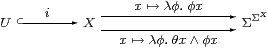
which is an example of the one in §6.5, with E≡λφ.θ∧φ. Notice that this is the same formula that we saw in §5.6 when we showed that open subspaces are Σ-split.
The question is therefore whether E is a nucleus. Expanding the λ-calculus definition in §6.7, we require
| Φ(λψ.ψ y∧θ y)∧θ y ⇔ Φ(λψ.ψ y)∧θ y. |
This follows from the Euclidean principle, putting σ≡θ y and F≡λτ.Φ(λψ.ψ y∧τ). Conversely, by considering Y≡1, θ≡λ y.σ and Φ≡λ G. F(G⊤), we see that this principle is also necessary.
Hence the Euclidean principle is exactly what we need to satisfy the abstract definition of nucleus. On the other hand, E satisfies the more user-friendly lattice-theoretic characterisation of nuclei that we also mentioned in §6.7, just using the distributive law. Of course, that is because the proof of this characterisation makes use of the Phoa principle (§11.6).
By a similar argument, λφ.φ∨θ is a nucleus (for the closed subspace coclassified by θ) iff Σ satisfies the dual Euclidean principle.
8.4.
We may therefore use the monadic framework in §6
to define the pullbacks in §7.1 and §7.4.
Then, bearing in mind that we still have to verify the stronger meanings
that these words have outside this paragraph,
we call an inclusion i:U↪ X open if it (is isomorphic
to one that) is the pullback of ⊤:1→Σ along some
(not â priori unique) θ:X→Σ, which classifies U.
In particular, θ≡⊤ classifies id:X↪ X.
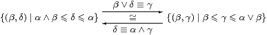
In order to prove that open inclusions form a dominion with dominance Σ in the sense of Rosolini (§7.3), one of the things that we have to show is that the composite of two open inclusions is open. For this, we use the Σ-splitting I that is provided by the monadic framework.
Suppose that V↪ U↪ X are classified by φ:ΣU and θ:ΣX respectively. Since I splits Σi, we have φ u⇔Σi(Iφ)u⇔(Iφ)(i u), so the bottom right square commutes:
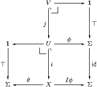
We claim that the rectangle on the right is a pullback, so Iφ classifies V⊂ X.
First, note that
| Iφ = (I·Σi· I)φ = E(Iφ) = θ∧ Iφ⊑θ. |
If x:Γ→ X and Γ→1 make a commuting quadrilateral with Iφ and ⊤ then ⊤⇔ Iφ x⇒θ x. So x=i u for some u:Γ→ U since θ classifies U, and φ u⇔(Iφ)(i u)⇔ Iφ x⇔⊤, so u=j v for some v:Γ→ V since φ classifies V. Hence x=(i· j)v, and v is unique since i· j is mono. We therefore have the composition property, and the inclusions V↪ U↪ X have classifiers Iφ⊑θ:X→Σ.
If U,V↪ X are open subobjects of X classified by θ,ψ:ΣX, and V⊂ U, then by the pullback property,
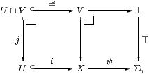
V=U∩ V↪ U is also an open subspace, classified by φ≡ψ· i≡Σiψ:ΣU, and we have the same situation again, with ψ=Iφ⊑θ.
Conversely, if ψ⊑θ:X→Σ then ψ=ψ∧θ=Eψ=Iφ where φ≡Σiψ. So the open inclusion V↪ X classified by ψ factors as V↪ U↪ X, where V↪ U is classified by φ. Hence we have an order-isomorphism between open subobjects V⊂ U↪ X and maps ψ⊑θ:X→Σ, from which it follows that classifiers are unique.
We are justified in calling i an “open” inclusion because I⊣Σi in the sense of §8.2, and the Frobenius and Beck–Chevalley laws (§2.9) hold [Proposition C 3.11]. If we want to use this result in the study of set theory (§3) then we must be careful not to assume that I preserves ⊑, but the same result also proves this. We write ∃i for I, for reasons that we explain in §8.7.
By reversing the order ⊑ throughout this argument and assuming the dual Euclidean principle, ⊥:1→Σ is a dominance too. We call the inclusions that are expressible as pullbacks of ⊥ along θ:1→Σ closed, say that θ co-classifies them and write ∀i for I. Beware, however, that if θ⊑φ classify C and D respectively then D⊂ C.
See §7 for an important converse result.
8.5.
In practice, it is often easier to reason with the Gentzen-style rules
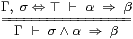
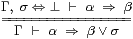
|
that are equivalent to the Euclidean principle and its dual, cf. §§2.1, 7.2 & 7.8.
To do this, we first have to modify the definition of contexts in §6.1, which now consist of both typed variables and equational hypotheses of the forms σ⇔⊤ and σ⇔⊥ for σ:Σ. We proved the Euclidean principle from the Gentzen rule on the left using such contexts in §7.2, and the dual is similar.
This modification is syntactic sugar (conservative). A context consisting of several variables and hypotheses of both kinds may be interpreted as a locally closed subspace (i.e. the intersection of a closed subspace with an open one) of the product of the types of the variables.
Using the Euclidean principle, the open subspace classified by σ is Σ-split with nucleus E≡λφ.σ∧φ. So the inequality α⇒β between subsubspaces is defined as α∧σ⇒β∧σ in the ambient space, which is what the Gentzen rule says.
These rules do not force F:ΣΣ to preserve the order — this has to be stated separately. Beware that we use this property so often in topology that we usually take it as read.
8.6.
Now we can ask when particular subspaces are open or closed,
starting with the diagonal X⊂ X× X.
It is natural to call X
For example, we expect ℕ and ℚ to have both properties (§9.5), and ℝ to be Hausdorff but not discrete (§11.10). This is in line with the computational fact that we may decide equality of integers or rationals, but only detect when real numbers are different.
Beware that, whilst points and the diagonal are open in a discrete space, arbitrary subspaces need not be. This is because the computable topology on the discrete space ℕ consists of the recursively enumerable subsets, not all of them. Also, our definition of Hausdorffness is slightly different from that in locale theory [Sim78] [Joh82, §III 1.3].
Classically, any discrete space is Hausdorff, but the proof employs a union that is illegitimate for us, and any free algebra with insoluble word problem provides a counterexample. Terms are equal iff they are provably so from the equations, so we observe equality by enumerating proofs, but none need be forthcoming. In particular, combinatory algebra (with a non-associative binary operation and constants k and s such that (k x)y=x and ((s x)y)z=(x z)(y z)) encodes the untyped λ-calculus, and therefore arbitrary computation, so equality of its terms is undecidable.
We use a subscript or brackets, n=X m or (n=m), to indicate the term of type Σ that this definition provides in a discrete space, with computable equality. This convention avoids ambiguity of notation with the underlying term calculus, in which any two terms of the same type may be provably equal or not.
The proof rules that relate these two notions of (in)equality are
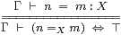
|
The rule for a Hausdorff space is not doubly negated: it is simply the way in which we express membership of a closed subspace, whilst ≠ is the natural name for its co-classifier.
From the Gentzen rules in §8.5, we obtain respectively
| φ x ∧ (x=X y) =⇒ φ y and φ x ∨ (x≠X y) ⇐= φ y. |
The usual properties of equality (reflexivity, symmetry, transitivity and substitution) follow from the first of these, whilst the dual argument gives the analogous properties of inequality. See Section J 4–5 for more detail in the setting of applications.
8.7.
Turning to compactness,
recall from §5.7 that it can be expressed
using an operator A:ΣΣX. This is Scott continuous
in the model (locally compact Bourbaki spaces),
but is simply a term or morphism in the axiomatisation.
It is enough to define a compact object K as one for which the map Σ→ΣK by σ↦λ k.σ has a right adjoint, ∀K, in the sense of §8.2. The two directions of the adjoint correspondence are exactly the introduction and elimination rules of the symbolic formulation, in which it’s more convenient to write ∀ k:K.φ k than ∀K(λ k:K.φ k).
However, in topology, we also have the dual Frobenius law (cf. §2.9),
| ∀ k.(σ∨φ k) ⇔ σ∨∀ k.φ k, |
for free, from the Phoa (or dual Euclidean) principle (§4), with F≡λτ.∀ k.τ∨φ k. This does not hold in intuitionistic set theory, but it was identified in intuitionistic locale theory by Japie Vermeulen [Ver94].
The first of the familiar properties of compact spaces is that any closed subspace i:C⊂ K is also compact. Its quantifier is given by ∀C≡∀K·∀i, where ∀i is the Σ-splitting of i in §§5.6 & 8.4 [Proposition C 8.3].
Products and coproducts of compact spaces are again compact, as are equalisers and pullbacks targeted at Hausdorff spaces [Sections C 8–9].
The Beck–Chevalley condition (§2.9) also comes for free, as substitution under λ [Proposition C 8.2]. Its lattice-theoretic interpretation is that any topology ΣX admits K-indexed meets, and not just finite ones (§7.9).
8.8.
When we try to apply these ideas to compact subspaces,
we find that the monadic framework in §6 does not provide
a sufficiently general theory (so it doesn’t extend to proper maps either).
This is related to the fact that,
in the leading model (§5.4),
a compact subspace of a non-Hausdorff locally compact Bourbaki space
need not itself be be locally compact.
This is discussed in
[Section G 5],
which is based on [HM81].
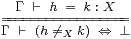
The clearest treatment for ASD is that in Section J 8, which exploits the fact that the main object of study in that paper is a Hausdorff space (ℝ), by restricting attention to subspaces that are both closed and compact. Since a Hausdorff space H has ≠, we expect the operator A:ΣΣH to represent (as a compact space) the closed subspace that is co-classified by
ω ≡ λ x.A(λ y.x≠ y)
if
 for any φ:ΣH.
|
If H is also compact, we obtain conversely
| Aφ ⇔ ∀ x:H.ω x∨φ x. |
Hence closed and compact subspaces coincide in a compact Hausdorff space, because there
| φ x ⇔ ∀ y:H.(x≠ y)∨φ y, |
which is obtained from the formula in §8.6. Notice that A, like θ (§8.4), decreases in the order (§8.2) as the compact or closed subspaces get bigger.
8.9.
To make sense of this equivalence between closed and compact subspaces,
however, we need some way of saying that K is “the same subspace” as C.
We do this by defining
| a∈ C as θ a⇔⊥ and a∈ K as A⊑λφ.φ a |
for any term a:X, possibly including parameters.
The definition of a∈ K is motivated by the idea in [HM81, Wil70] that a compact subspace is the intersection of its open neighbourhoods. In a non-Hausdorff space, however, this intersection may be larger than the original compact subspace, and is called its saturation. Nevertheless, C and K do have the same “elements” according to the definitions that we have just given. The account in Section J 8 also treats direct images and compact open subspaces.
8.10.
Because of the lattice duality of the axioms that we have introduced
so far (§§7.8f), there is a dual notion to compactness.
We call it overtness, and it is related to the existential
quantifier.
By the same arguments as for compact Hausdorff spaces [Sections C 6–9],
See [Section C 8 & 10] for the proofs, which were inspired by similar results in [JT84]. We spell out the last part, as it will be important later. Define
| F:ΣX→ΣY by Fφ ≡ λ y:Y.∃ x:X.φ x∧(f x=Y y). |
Then Fφ(f x) ⇔ ∃ x′:X.φ x′∧(f x′=Y f x) ⇔ ∃ x′:X.φ x′∧(x′=X x) ⇔ φ x by §8.6.
Hence f:X↣ Y is Σ-split, and X≅{Y ∣ E} by §6.8, where E≡Σf· F. Expanding E, we find that X⊂ Y is the open subspace classified by θ (§8.3).
8.11.
We have made a lot of use of the analogy between (Stone duality for)
set theory and topology.
This is no longer applicable in the case of partial maps,
where the Phoa principle makes the topological account much simpler
than the set-theoretic one [D].
In Rosolini’s theory of dominions and dominances (§7.3), a partial map (i,f):X⇀ Y consists of an “open mono” i:U↪ X and an (ordinary or “total”) map f:U→ Y.
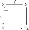
Then Y↪ Y⊥ is a partial map classifier or lift if, for every partial map X⇀ Y, there is a unique total map X→ Y⊥ that makes the square a pullback. In particular, 0⊥=1, 1⊥=Σ and Σ⊥=ΣΣ, but this coincidence ends there.
Classically, as the notation suggests, Y⊥ is obtained by adding a single point ⊥ to Y, to serve as the “undefined” value of f x for x∉ U. In topology, when U⊂ X is Scott open, and in particular upper, ⊥ must lie below Y in the order. In intuitionistic set theory, on the other hand, we need higher order logic to define Y⊥⊂℘(Y) as “the set of subsets with at most one element”.
Using the monadic framework and the Phoa principle, we obtain Y⊥ in a much simpler way via its topology. This forms a comma square,
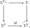
which is defined like a pullback except that the order ⊑ replaces equality in the bottom right. So
| ΣY⊥ ≡ {(ψ:ΣY,σ:Σ) ∣ σ⇒ψ y} |
in set-theoretic notation. Since this is a retract of ΣY×Σ, we may also construct the comma square in this way in ASD.
We also need to define the Eilenberg–Moore algebra structure on ΣY⊥ and prove the universal property of Y⊥. The latter involves maps X→ Y⊥, which are homomorphisms out of ΣY⊥, whereas the definition of a comma square uses incoming maps. It’s not difficult to prove the result using Scott continuity, but without this it’s rather delicate. The key idea is the isomorphism
that follows from distributivity, but is actually a weaker property called modularity that holds in many lattices of subalgebras, such as those of groups and vector spaces.
8.12. This comma square construction is a special case of Artin gluing,
which recovers the topology of a space from those of an open subspace
and its closed complement, together with a map that encodes the
way in which these fit together [AGV64, Exp. IV §9.5].
However, the general version of Michael Artin’s construction does not work in ASD, because it is computable topology and so inherits some of the strange behaviour of computability theory. In particular, the open (RE) subspace of ℕ consisting of codes of terminating programs does not glue to its closed (co-RE) complement in anything like the Artin fashion [Section D 4].
The special case of the lift is also known is topology as the scone (Sierpiński cone) and in topos theory as gluing or the Freyd cover. See [Tay99, §§7.7 & 9.4] for further mathematical and historical discussion.