


In the previous section we described a number of properties in topology that are related to the monadic adjunction Σ(−)⊣Σ(−). We also showed that this is satisfied when Σ is the Sierpiński space in the category of locally compact spaces, or the subobject classifier in any topos, and in these cases ΣX is the topology or powerset of X. In this section we describe the purely categorical structure that we abtract from this situation. Then we shall show how it can can be formulated as a new symbolic language. See [A][B] for the details in ASD and [BW85, §3.3] [Mac71, §VI 7] [Tay99, §7.5] for textbook accounts of Beck’s theorem.
In investigating this structure, we shall need to apply the (contravariant) functor Σ(−) repeatedly, giving some unwieldy towers of exponentials. For this reason, we often write
| Σ2 X ≡ ΣΣX Σ3 X ≡ ΣΣΣX Σ4 X ≡ ΣΣΣΣX … |
The unit of the adjunction, ηX:X→Σ2 X, is the transpose of the co-unit, εX≡evX:ΣX× X→Σ, which is in turn the other transpose of id:ΣX→ΣX. Then η is part of the structure of the monad, for which Σ2 X is the free algebra on an object X, with structure map µX≡ΣηX, where µ is called the multiplication.
The corresponding symbolic language is the familiar one with pairing and λ-abstraction, except that the exponential type SX and corresponding λ-terms λ x.s may only be formed in the case where S (the type of the body s), is a power of Σ. Then
| ηX x≡λφ.φ x and µXΦ≡λ x.Φ(λφ.φ x) |
are the unit and multiplication of the monad. Contexts (§2.6) in this first prototype (§3.2) of the language just consist of typed variables, but the study of recursion will oblige us to add equational hypotheses §§8.5 & 9.10.
6.2.
The first clause of Beck’s theorem (§5.5(a)) says that
if Σf:ΣY→ΣX is invertible
then so already was f:X→ Y.
This is equivalent to requiring, for every object X, that
ηX be the equaliser of the parallel pair in the diagram,
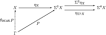
In other words, if P also has equal composites then there is a unique map that makes the triangle commute.
P has equal composites iff its transpose, ∼ P:ΣX→ΣΓ, is a homomorphism of Eilenberg–Moore algebras for the monad. Sobriety then says that ∼ P=ΣfocusP (Section A 4).
6.3.
According to the technique of §2.8,
a morphism P:Γ→Σ2 X
is the same thing as a term Γ⊢ P:Σ2 X.
This has equal composites with the parallel pair above iff
| Γ, Φ:Σ3 X ⊢ Φ P = P(λ x.Φ(λφ.φ x)):Σ. |
We call P prime if this holds, extending the usage of this word beyond that in §4.1.
Here we have our first example of the difference between the definitions that we give for the foundations and those that are appropriate for the applications (§3.8): when we add the other topological structure to the theory, primality can be characterised more simply by saying that P preserves ⊤, ⊥, ∧ and ∨ (§11.6).
The object X is sober iff every prime P has a unique fill-in
| Γ ⊢ focusP:X such that Γ, φ:ΣX ⊢ φ(focusP) = Pφ:Σ. |
Following §2.11, we turn this universal property into a new system of symbolic rules. Indeed, we have just given the introduction and β-rules for focus (Section A 8).
The operation in the elimination rule takes a:X to λφ.φ a:Σ2 X. This is prime: categorically, ηX has equal composites with the parallel pair, by naturality of η(−) with respect to ηX, but one could also check this by a λ-calculation. Finally, the η-rule is focus(λφ.φ a)=a:X.
The normalisation theorem (cf. §2.12) says that focus may be eliminated from any term φ:ΣX, whilst any term of ground type is provably equivalent to focusP, where P does not itself involve focus.
The symbolic calculus extended with focus corresponds (via §2.8 again) to a certain category. By the normalisation theorem, this has the same objects (contexts) as the original one, but its morphisms Γ→Δ are in bijection with the Eilenberg–Moore homomorphisms ΣΔ→ΣΓ (Section A 6–7).
6.4.
It is pertinent to ask of this β-rule how much of the expression
surrounding focusP is to be taken as φ, and moved
inside Pφ. That is, for any F:ΣΣ, does
| F(φ(focusP)) become F(Pφ) or P(λ x.F(φ x))? |
So long as P is prime, this doesn’t matter, because the two results are equal (consider Φ≡λ Q. F(Qφ) in the definition of primality).
Hayo Thielecke [Thi97] considered an operation called force with the same β-rule, but without the primality side condition. Now it does matter where we draw the boundary of the super-term φ: the computational effect is to pass φ as an argument to P, and then jump to the continuation F when (if) P returns. In order to study computational effects in general, Thielecke developed categorical machinery that is very similar to our account of abstract sobriety, but independently.
6.5.
The second clause of Beck’s characterisation (§5.5)
brings in all algebras that are definable in the
sense of Eilenberg and Moore.
It says that certain equalisers exist,
and are taken by Σ(−) to coequalisers
(Section B 2–4).
Our approach to this is to spell out what was meant in §5.5 by “data on Y that ought to define a Σ-split subspace”. For this, it is enough to consider equalisers of the form
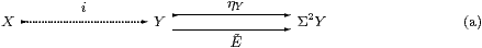
that become split by ηΣY when we apply Σ(−). This means that, in the diagram
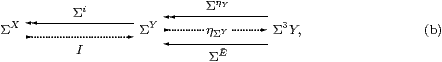
the equation ΣẼ·ηΣY·ΣẼ = ΣẼ·ηΣY·ΣηY holds.
Besides asking for the equaliser i:X↣ Y in (a), we further require that the solid lines in diagram (b) form a coequaliser. For this we simply need a map I such that
| I·Σi = E ≡ ΣẼ·ηΣY. |
Whilst these conditions may look very strange, they are actually adapted from the definition of an Eilenberg–Moore algebra (A,α): with Y≡ΣA, Ẽ≡Σα and I≡ηA, they yield P A≡ X. Conversely, one can show that the category of algebras admits coequalisers of this form. However, the category of spaces that we have axiomatised here need not have all equalisers, for example LKLoc does not.
6.6.
Beck’s theorem requires the map Ẽ to satisfy a certain equation.
Writing this in the λ-calculus (§2.8),
we call E:ΣY→ΣY a nucleus if
| Φ:Σ3 Y, y:Y ⊢ E(λ y′.Φ(λψ.Eψ y′))y = E(λ y′.Φ(λψ. ψ y′))y, |
observing the extra E on the left hand side. Since we don’t want to deal with dependent types, we do not allow E to have parameters.
We have appropriated the name “nucleus” from locale theory (§4.8), since both kinds of nuclei are used to define subspaces. The definitions are not the same, but the use of different letters (E and j) should avoid ambiguity. Like primes (§6.3), nuclei in ASD have another characterisation in the presence of the full topological structure (§11.6), namely
| E(φ∧ψ)= E(Eφ∧ Eψ) and E(φ∨ψ)= E(Eφ∨ Eψ). |
In this setting, ASD nuclei are Scott continuous, whilst those in locale theory need only be monotone; on the other hand, localic nuclei satisfy id⊑ j, which is not required in ASD. Beware in particular that the ASD nucleus for an open subspace is given by Eφ≡(θ∧φ) (cf. §5.6), whilst the localic nucleus is jφ≡(θ⇒φ) (§4.8). Nevertheless, there are some important examples that satisfy all of the conditions of both definitions [Section I 8] [L].
6.7.
The symbolic calculus (§2.11) that corresponds to Beck’s theorem
has to define both the equaliser of the main types
and also the coequaliser of their topologies.
It does this using two sets of rules
(Section B 8).
A term Γ⊢ a:Y has equal composites with the parallel pair in §6.5(a) iff
| Γ, ψ:ΣY ⊢ ψ a = Eψ a:Σ, |
and then we say that it is admissible. The introduction rule for the equaliser, i.e. its universal property, then allows us to form
| Γ ⊢ admita:{Y ∣ E}, |
whilst the inclusion i is the elimination rule. The β- and η-rules are
| Γ ⊢ i(admita) = a:Y and x:{Y ∣ E} ⊢ admit(i x)=x:{Y ∣ E}. |
We also have to ensure that the second diagram (§6.5(b)) is a coequaliser, using another set of rules. We get the introduction rule for free, as the map Σi:ΣY→Σ{Y ∣ E}. The elimination rule says that Σi is split by another map I,
| y:Y, ψ:ΣY ⊢ IY,E(λ x:{Y ∣ E}.ψ(iY,E x))y ⇔ Eψ y, |
so I·Σi=E and Σi· I=id{Y ∣ E}. These equations are the β- and η-rules
| y:Y, ψ:ΣY ⊢ I(λ x.ψ(i x))y = Eψ y |
and
| x:{Y ∣ E}, φ:Σ{Y ∣ E} ⊢ Iφ(i x) = φ x. |
The normalisation theorem for this calculus (cf. §2.12) says that every type can be embedded as a subspace of a type formed without comprehension, and terms also normalise in a simple way. This makes the corresponding category equivalent to the opposite of the Eilenberg–Moore category (Section B 9–10).
6.8.
Any map f:X→ Y that is Σ-split,
i.e. with F:ΣX→ΣY such that F·Σf=idΣX
or Fφ(f x)=φ x, agrees up to isomorphism with
the subspace {Y ∣ E} with E≡Σf· F.
In particular, f is regular mono.
The isomorphism is
|
To show that these maps are mutually inverse, we need the rules above, together with
| i(focusX P) = focusY(Σ2 i P), |
first proving that if P is prime then so is Σ2 f P. This uses sobriety of X and Y.
6.9.
Notice that the Σ{}β-rule
is the only one that introduces E into terms.
This is something that we want to avoid if at all possible,
because the expressions for nuclei are usually very complicated.
When E does find its way into a program,
it will give rise to a substantial computation.
Actually, this is what we expect from practical considerations. Consider, for example, the nucleus that defines ℝ in ASD (§5.12). The universal quantifier that says that the interval is compact is given by
| (∀ x:[0,1].φ x) ≡ Iφ(λ d.d< 0, λ u.u> 0), |
which applies the extension Iφ of φ to the pseudo-Dedekind cut that represents the interval. The normalisation theorem introduces the expression E, in this case the one given in §5.12. This divides the interval up into sufficiently small parts, on each of which the predicate φ must be satisfied, but in the fashion of Ramon Moore’s interval analysis [Moo66], i.e. by evaluating the arithmetical operations on the (endpoints of) the subinterval, instead of using single real values [Bau08][I][K].
6.10.
How common is the monadic situation?
We may obtain it from any category S0 with an object Σ0
that has powers Σ0X.
Let A be the Eilenberg–Moore category for the monad on S0;
then S≡Aop has the monadic property.
The proof of this is very easy — apart from the most basic requirement,
namely that S have products (coproducts of algebras)
(Section B 7).
Can other categorical structure be defined in S, before we add specifically topological features? We have already remarked in §5.3 that colimits come for free, as long as we have the corresponding limits, so S has coproducts and Σ-split coequalisers. In fact, the coproducts are stable and disjoint, i.e. the category S is extensive (cf. §9.1). Note that 0↣1 is Σ-split iff Σ has a point (§6.1(b)). Whilst extensivity is a purely categorical statement, its proof relies heavily on the new λ-calculus (Section B 11).
6.11. Thielecke argues that Σ (the “answer type” R, in his notation)
needs no extra structure.
In his view, it may perhaps be seen as a free type variable,
or one that is quantified at the outermost level.
I once said to him that his work
must therefore be either very superficial or very deep.
The fact that one can develop quite a lot of theory
from just this monadic adjunction Sop⇆S,
or from pure equideductive logic (cf. §12.5), without any other hypothesis on Σ,
leads me to believe more and more in the second possibility.
This structure and its generalisation (cf. §12) will provide the skeleton on which the more obviously topological structure is the flesh. Dressed in a different way, I also believe that it could be applicable to game semantics of sequential computation, algebraic geometry, differential geometry and quantum logic.
6.12. Our use in §6.7 of the traditional notation {Y ∣ E}
for subset formation advertises more than it can deliver
on the basis of the monadic hypothesis alone.
Although the symbolic formulation is a little easier to handle than the categorical one, it has to be said that devising nuclei in ASD requires a lot of inspired guesswork, because of the need to find splittings. However, this problem is by no means a new one: it is a feature of Jon Beck’s theory of monads that he inherited from his own inspiration in homological algebra, where we cannot in general split short exact sequences. This had in turn come from the (mathematically interesting) fact that there are non-split extensions of Abelian groups, starting with the cyclic group of order 4.
Like the category of locally compact spaces, S need not be cartesian closed. However, when we develop induction and recursion in §9, we find that the lack of general equalisers is the real handicap to developing the theory. The conjectural extension that we begin to investigate in §12 would provide a much more expressive language in the notation {y:Y ∣ ⋯}, without the need for splittings. It would also provide general equalisers and function spaces. Nevertheless, splittings, where they exist, will remain important, for example to prove that [0,1]⊂ℝ is compact (§5.12).