


This section requires more work, and in particular §§12.10ff should be replaced by a less technical conclusion that describes my current plans.
In the HTML version it has not been possible to make the necessary distinction between symbols. Please read the DVI, PDF or PostScript version for the correct formatting.
As we said in §3.7, any generalisation of ASD must go way beyond the category of Bourbaki spaces. This section describes some investigations I am conducting while I write this story, so it therefore involves empirical tests, and carries significant risk of failure (§3.9). Indeed, this is just what has happened to several previous attempts to find models.
12.1.
Curiously, one way of extending the traditional categories to
have all exponentials is to add new colimits,
specifically quotients of equivalence relations.
The new objects, as proposed by Dana Scott,
are called equilogical spaces [BBS04]
.
Giuseppe Rosolini put them in a sheaf-like categorical framework
[Ros00]
that also includes Martin Hyland’s earlier filter spaces
[Hyl79],
and there also a cartesian closed extension for locales
[Hec06].
Countably based equilogical spaces form a full subcategory
of Bourbaki spaces [MS03].
The equivalence relations in these constructions are not obliged to respect the topological structure in any way. For example, the four-point object that identifies ⊥ of one copy of the Sierpiński space with ⊤ of another has four open subspaces, but also a discrete two-element subspace, one of whose open subsubspaces cannot be extended to the whole space. Such objects owe more to set theory than to topology, but we can modify Scott’s construction to eliminate them.
12.2. When we considered recursion in §9.8,
the main defect that we found in the monadic framework of §6
was not the lack of function spaces, but that of general equalisers.
This was also the main problem in defining the compact subspace K⊂ X
that corresponds to a modal operator A:Σ2 X (§8.9):
we should have K≡{x:X ∣ A⊑λφ.φ x},
which is the equaliser of λφ.Aφ and λφ.Aφ∧φ x.
We adopted an ad hoc solution to this in §9.10, adding a second category L that has equalisers but not all powers of Σ. It does have some additional function-types, in particular ℕℕ and ℝℝ, but not ℕℕℕ or ℝℝℝ.
Plainly the natural step is to ask for both equalisers and powers of Σ. This simple hypothesis already leads to some interesting observations: a complicated subtype such as
| {x:X ∣ f x = g x:Σ{y:Y ∣ p y = q y:ΣZ}} |
invites re-writing as {x:X ∣ ∀ y:Y.(∀ z:Z.p y z = q y z)⇐(f x y = g x y)} . Here ∀ is a new kind of universal quantifier that, at first, we keep separate from ∀ for compactness (cf. §12.6). Also, whilst we have taken ∀ to bind more tightly than ⇒, the scope of ∀ includes ⇐ but is terminated by ⊢.
12.3.
Let’s put this a bit more precisely.
As in §6, the lattice structure of the object Σ
is not used in the fundamental construction,
so it could perhaps be replaced by a different kind of algebra.
Consider any equaliser i:E↣ X⇉ΣY in a category S with all finite limits and powers of an object Σ. Then, for any a:Γ→ X such that the composites Γ× Y→ X× Y⇉Σ are equal, there is a unique b:Γ→ E such that a=i· b.
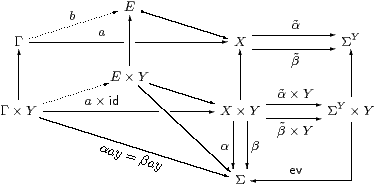
This property, which is called a partial product, is of interest because it can be stated entirely within any full subcategory L⊂S that is closed under products and regular monos, by which we mean equalisers targeted at objects of S that need not belong to L.
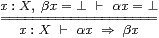
Following our method (§2.11), we can rewrite this categorical idea syntactically,
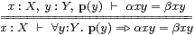
|
where p denotes a regular mono into Y. This generalises the diagram to allow the Y there to be the result of a similar construction, and justifies the informal usage above. By a small modification to the diagram, it is easy to show that we may substitute for the free variable x under this quantifier, cf. §2.9.
Since taking the product of the targets of the equalisers provides the intersection of two regular monos, the logic also has conjunction, for which we write &. Then we have
| ∀ y. p(y) ⇐ (∀ z.q(z)⇐α x y z=β x y z) ⊣⊢ ∀ y z.p(y) & q(z) ⇐ α x y z=β x y z, |
which also gives a meaning to ∀ y.p(y)⇐r(x,y), so long as r(x,y) is formed using ∀⇐, &, ⊤ and equations.
12.4.
Notice that, whilst it may range over any type,
because we have not allowed the target ΣY to be a dependent product.
One reason for avoiding dependent products is of course that they make things much more complicated, both categorically and syntactically. This restriction may therefore be loosened if we can construct examples of such products, or show that they are consistent. A situation in which we might reasonably expect to do that is indexing over ℕ, or more generally over any space that is either discrete or Hausdorff.
If you come from a type-theoretic background, you may be tempted to think, “this guy’s just a categorist, we don’t have any problem with dependent types”, but I would point out that I have written a PhD thesis and a book on this topic [Tay86, Tay99], mentioned in §2.6. If you insert parameters into formulae without considering what they mean topologically, you are just being another logician who dictates foundations to mathematicians (§1.1).
We cannot have dependent products in their full generality if we want to do topology rather than set theory (cf. §2.9). A category with unrestricted dependent products is called locally cartesian closed; since the exponentials are right adjoint to pullback, the latter preserves arbitrary colimits, in particular epis.
For example,
we write ϖ for the ascending natural number domain,
in which the topological order agrees with the arithmetical one,
and Scott continuity creates a top element, so
0⊑ 1⊑⋯⊑∞,
as illustrated on the left:
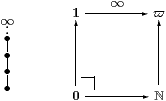 Then ℕ→ϖ is epi
(in fact Σϖ↣Σℕ is split mono),
but not surjective, since ∞ has no inverse image,
i.e. its pullback is the initial object.
Then ℕ→ϖ is epi
(in fact Σϖ↣Σℕ is split mono),
but not surjective, since ∞ has no inverse image,
i.e. its pullback is the initial object.
Therefore, a category of “sober” spaces and Scott-continuous functions cannot be locally cartesian closed.
12.5.
The new fragment with ∀⇐, ⊤ and & is called
equideductive logic.
Although it is rather feeble, it is interesting for a number of reasons.
Besides being a pun on Scott’s word, the name is justified because
this is how we reason with proofs of equations in algebra.
Each judgement
| x:X, y:Y, …, a=b, c=d, … ⊢ e=f |
becomes
| ∀ x:X.∀ y:Y.… a=b & c=d & ⋯ ⇐= e=f. |
Here, all of the variables are bound by ∀, but it’s natural to relax this, using free variables of the new calculus in place of terms on the right of ⊢ that were previously metavariables in proof rules. The rule for ∀⇐ does, however, oblige us to bind all variables that occur in the equational hypotheses a=b, etc. , but this seems to be natural. The horizontal line of a proof rule becomes another ⇐, and the metavariables of the rule are bound by its ∀.
The bonus is that equideductive logic allows us to nest ⇐ arbitrarily deeply. We may write induction as
| ∀ n. p(0) & (∀ m.p(m) ⇐ p(m+1)) ⇐= p(n), |
in which p(n)≡∀ x:X.⋯ is the property to be proved. Note that, because of the variable binding rule, the variable n can only occur in the equation at the right-hand end of p(n). (Recall from §12.3 how implications between predicates are reduced to a form with an equation on the right.)
If it is possible to relax this rule, allowing m on the left of the innermost ⇐ below, we may express course-of-values induction or well-foundedness of < as
| ∀ n. (∀ m. (∀ k. k< m⇐p(k)) ⇐ p(m)) ⇐= p(n). |
Equideductive logic may be interpreted in the category of (sober) Bourbaki spaces, in the obvious way, namely by quantification over sets of points. However, having identified it categorically as a partial product, we may look for other semantic interpretations. These might include the category of locales or formal topology, but this is not clear.
In any model such as these, there are accidental containments between regular monos, represented syntactically by judgements p(x)⊢q(x) that need not follow from the axioms. In what follows, we shall understand the calculus in a purely syntactic way, without allowing particular concrete interpretations to impose accidental judgements over which we have no control. After that, we can add new axioms according to our own purposes (§12.11).
12.6.
Combined with the lattice structure on the Sierpiński space,
equideductive logic is also just what we need to form open, closed,
compact and overt subspaces in ASD.
Some of the following examples were first observed by Matija Pretnar.
As in §8.2, we use ⇒, ⊑ and ⊑ for the order relation that arises from the lattice structure on Σ. The Gentzen rules (§8.5) relate these orders to the new implication. Starting from these rules in the form
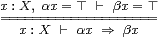 and
and
|
the translation above yields
| (∀ x.α x=⊤⇐β x=⊤) ⇔ (∀ x.α x⇒β x) ⇔ (∀ x.β x=⊥⇐α x=⊥). |
Also recall that, via λ-abstraction, the bottom line of the rules is the the definition of α⊑β.
This means that we may interpret any term α:ΣX as an equideductive predicate ∀ x.α x=⊤, the corresponding regular mono being an open inclusion (cf. §7.2). Then the lattice order relations ⇒, ⊑ and ⊑ are special cases of ⇐. Similarly, the rules for ∧ and ∨ say that ∧ is a special case of &:
| α=⊤ & β=⊤ ⇔ α∧β=⊤ and α=⊥ & β=⊥ ⇔ α∨β=⊥. |
Recall that =N in a discrete space N (§8.6) was also a special case of general equality of terms,
| n=m ⇔ (n=N m)=⊤, whilst h=k ⇔ (h≠H k)=⊥ |
in a Hausdorff space H. The quantifier ∀ in a compact space is related in a similar way to our more general quantifier ∀, cf. §5.7:
| (∀ x. φ x=⊤) ⇔ (∀ x.φ x)=⊤, whilst (∀ x. φ x=⊥) ⇔ (∃ x.φ x)=⊥ |
in an overt space.
12.7. We can therefore just use the traditional symbols
=, ∧, ⇒ and ∀,
without the variants =N, &, ⇐ and ∀, but they generate two different logics:
We may form =, ≠, ∀ or ∃ within the inner calculus so long as the relevant space is discrete, Hausdorff, compact or overt, as before. The other cases, including ⇒, take us to the outer calculus.
By an idea that has seen many uses in logic, the formulae
| (p⋎q)(a) ≡ ∀στ:Σ. (∀ a′.p(a′)⇐σ=τ) & (∀ a″.q(a″)⇐σ=τ) ⇐ σ=τ |
and
| (∃ x.p)(a) ≡ ∀στ. (∀ a′ x.p(x,a′)⇐σ=τ) ⇐ σ=τ |
extend ∨ and ∃ from terms of type Σ to general predicates. However, they only obey the distributive and Frobenius laws
| (p⋎q)( |
| ) & r( |
| ) ⊣⊢ ((p&r)⋎(q&r))( |
| , |
| ) and (∃ x.p)( |
| ) & r( |
| ) ⊣⊢ (∃ x.p&r)( |
| , |
| ) |
when the variables a and b are disjoint. Also, unlike their powerful namesakes in intuitionistic logic, they do not allow us to recover a witness for ∃, or knowledge which disjunct (p or q) was true.
12.8.
Since we defined ∀⇐ in §12.3
from equalisers of exponentials, we may form subspaces using comprehension,
and terms belong to the subspace iff they satisfy the defining predicate.
Unlike the nuclei in §6,
these may be manipulated in a way that is very similar to set theory
.
In particular, open, closed, compact and overt subspaces of X are given by
| {x ∣ θ x=⊤}, {x ∣ θ x=⊥}, {x ∣ ∀θ.▫θ⇒θ x} and {x ∣ ∀θ.θ x⇒◊θ}. |
We can use the arbitrarily nestable implications in equideductive logic to write more complicated definitions in general topology. For example, the overt subspace I⊂ X defined by a modal operator ◊ is connected (Section J 13) if
| ◊⊤ ⇔ ⊤ and …, φ,ψ:ΣX, φ∨ψ=⊤I ⊢ ◊φ∧◊ψ ⇒ ◊(φ∧ψ). |
In the new notation, where I≡{x:X ∣ ∀θ.θ x⇐◊θ}, the second part of this becomes
| ∀φ,ψ. (∀ x. (∀θ.θ x⇐◊θ) ⇐ φ x∨ψ x) ⇐= (◊φ∧◊ψ⇒◊(φ∧ψ) ). |
Unfortunately, the variable-binding rule means that this formulation can only be used when ◊ has no parameters, whereas these were an important feature of the treatment of the solution of equations in [J]. As we said in §12.4, we would hope to allow discrete or Hausdorff parameters in a future generalisation. However, before you dismiss this as a defect of the calculus, you should think carefully whether it might be telling us something about the topology of the connected components of, for example, the zero-set of a function.
12.9.
We are running ahead of ourselves: although we introduced
equideductive logic as a necessary feature of
a category with both exponentials and equalisers,
we still have to show that it is sufficient.
In fact, it provides exactly the abstract basis that is
needed to construct (a version of) Scott’s category of equilogical spaces.
As in §6, this construction is independent of the lattice structure
on Σ.
We start with some urtypes that play the role of unions of algebraic lattices, closed under product and Σ(−). It is convenient to assume that they also admit stable disjoint sums, although these could be eliminated in what follows by using lists of urtypes instead. The urterms are generated from variables and certain combinators, for which we assert equations of type Σ as equideductive axioms without ⇐.
Then an equideductive space X is a triple (A,p,q) where A is an urtype, p is a predicate in this logic on ΣA, and q one on A, for which
| φ,ψ:ΣA, p(φ), (∀ a:A.q(a)⇐φ a=ψ a) ⊢ p(ψ). |
The left hand side of this is essentially the partial equivalence relation φ∼ψ in Scott’s construction. Hence X is represented as a partial quotient of ΣA; in particular 1=(0,⊤,⊤) and Σ=(1,⊤,⊤).
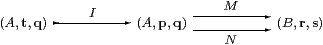
A function M:X≡(A,p,q)→ Y≡(B,r,s) is an equivalence class of urterms M:ΣA→ΣB such that
| φ:ΣA, p(φ) ⊢ r(Mφ) |
and
| φ,ψ:ΣA, p(φ), ∀ a.q(a)⇐φ a=ψ a ⊢ ∀ b.s(b)⇐ Mφ b=Mψ b, |
where M1=M2 if
| φ:ΣA, b:B, p(φ), s(b) ⊢ M1φ b=M2φ b. |
We have to make full use of the rules of the logic, including substitution under ∀ and the condition relating p and q for a space, just to prove that this is a category, S. Then the product is
| (A,p,q) × (B,r,s) ≡ (A+B, p·π0&r·π1, [q,s]), |
where [q,s] is the predicate on A+B given by q on A and s on B. The equaliser
is given by
| t(φ) ≡ p(φ) & (∀ b:B. s(b)⇐ Mφ b=Nφ b). |
Finally, for X≡(A,p,q) the exponential ΣX is given by (ΣA,qp,p), where
| qp(F) ≡ ∀φ,ψ:ΣA. p(φ) & (∀ a:A.q(a)⇐φ a=ψ a) ⇐= Fφ=Fψ. |
Since the category has all finite limits and powers of Σ, it has an interpretation of equideductive logic and the examples that we have given. There is a syntactic criterion on p and q that characterises when (A,p,q) is definable using this structure, and we restrict the notion of equideductive space to these objects. General exponentials and other categorical operations may be derived from this.
If Σ≡(1,⊤,⊤) is a lattice and satisfies the rules in §12.6 then it is a dominance, so we may reproduce (some of) the abstract topology in §8.
12.10.
This is a very pretty picture, but it is misleading,
as serious problems remain.
As we have seen, we must take a lot of care over the variable-binding rule.
It would be nice to weaken this, but its alternative may be more
difficult for customers (i.e. mathematicians who are interested in the
applications of topology, rather than logic itself) to use,
in contrast to the clear topological motivation for only allowing
∀ over compact subspaces.
The similarity with set theory should also serve as a warning of a more fundamental issue for the new calculus. As it stands, it is neither an extension of the letter of ASD as set out in §6, nor faithful to its spirit in ensuring that the objects that we construct have the right topology.
Take, for example, the “compact” subspace K≡{x:X ∣ ∀φ.▫φ⇒φ x}⊂ X that is defined by a modal operator ▫. Is K actually a compact space, with its own universal quantifier ∀K:ΣK→Σ? This is a problem that we could dodge in [J] because that studied a Hausdorff space (ℝ), where all compact subspaces are closed. Categorically, the inclusion i:K↣ X induces a map ΣΣi:ΣΣK→ΣΣX. For K to be compact, we need to find ∀K:ΣΣK that this map takes to our given ▫:ΣΣX. The theory should then relate parametric modal operators to proper maps, showing that these obey the Beck–Chevalley condition (2.9) and descent properties.
Another way of seeing this issue is that ∀K is a total function that it is convenient, both mathematically and computationally, to represent by the partial function ▫. This is similar to a long-standing problem in recursion theory, concerning definable total maps of higher type such as ℕℕ→ℕ or ℝℝ→ℝ. Amongst many authors, Hyland and Bauer studied it in their settings of filter and equilogical spaces [Hyl79, BBS04].
Applications in functional analysis also have something to say about this. Typically, a space X in this subject is not locally compact, so the space C(X) of continuous functions X→ℝ cannot be the exponential ℝX in the category of Bourbaki spaces. When I have asked analysts what “the right” topology on C(X) might be, they have said that there are horses for courses. Since X often carries either a metric (norm) or a measure (integration), there are various topologies on C(X) defined from norms and semi-norms that are useful for different purposes.
Is there perhaps a fundamental topology on YX, for which the others are continuous additional structure? So long as we can at least agree to exclude the discrete one, the clear candidate is the point–open or weak*-topology, which is the weakest or coarsest one for which each evx:YX→ Y is continuous. This means that the topology on YX is generated as an algebra by all of the λ f.φ(f x) for φ:ΣY and x:X.
Finally, we repeat that our category of equideductive spaces does not necessarily satisfy the sobriety and monadicity properties in §6.
12.11.
There is an unambiguous, if rather tedious,
procedure for investigating questions such as these.
Consider, for example, a modal operator ▫ on an equideductive space (A,p,q). This is given by a certain urterm, of type Σ3 A. From this we may compute the subspace K as an equaliser (A,t,q), and then also Σ2 X and Σ2K. The formulae for these are not very pretty, but the inclusions i:K↣ X and Σ2 i are realised by the identity, so ∀K, if it exists, has the same urterm as ▫.
The question is therefore whether this satisfies the equideductive properties that are required of a function ΣK→Σ. We write the hypotheses at the top of the page, the conclusion at the bottom and try to fill in the proof in between. In general, there need be no such proof using the abstract rules of the calculus, and nor need the property follow from the accidental judgements that hold in any particular model, such as Scott’s original equilogical spaces.
This is where an abstract approach wins over a preconceived set-theoretic model, as we have left open the option to add more axioms. You can’t fill in the necessary proof? No problem. Just add it as an axiom.
There is, of course, a price to pay for doing this. The resulting system may be inconsistent, in the sense of being able to prove undesirable theorems like 0=1. Indeed, since we have already got a complete axiomatisation of computably based locally compact spaces, we don’t want any additional equations to be provable for them. In terms of the construction of the category of equideductive spaces, we don’t want any new equations between urterms without hypotheses.
For equideductive logic, its weakness is its strength , as we can easily apply some proof theory to it. In particular, using the analogy between propositions and types (§2.2), proofs in this fragment may be considered as typed λ-terms, and strongly normalise (§2.3). They also have a domain-theoretic interpretation [HP89], in which Scott continuity corresponds to the proof-theoretic observation that, in a proof whose conclusion is an equation, any ∀-formula that occurs as a hypothesis must be used by instantiation at finitely many terms. This suggests a technique for rearranging the proof of the hypotheses of an instance of an additional axioms into one of its conclusion, thereby demonstrate the conservativity of the new principle.
12.12. This may make a profitable architectural practice,
but it’s not good science.
According to Karl Popper, we must lay down a theory that is coherent
in itself, and put our head on the block with a prediction that
is open to falsification.
That is what ASD did for the Heine–Borel theorem (§5.12).
A new axiomatisation should state both its principles and its applications
in its own language, not in some encoding,
which is what the construction in §12.9 provides.
For example, functional programming languages such as Haskell
[HHPJW07] add expressiveness by developing the mathematical
theory, not by taking short cuts in the underlying C implementation.
The principle for doing this was laid down by Galileo in his rejection of Aristotle: we assume that the universe beyond our own reach obeys the same laws as hold in familiar places. This has been applied many times in mathematics, in particular to successive generalisations of numbers and spaces: the complex numbers were introduced to solve quadratic and cubic equations, but otherwise their arithmetic agrees with the reals. In recursion theory, Scott continuity is a theorem for ground types, so we adopt it as an axiom for higher types (§9.13), which are “beyond our reach” in the sense that actual computation cannot proceed when there are free variables.
The criterion by which we regard certain territory as familiar and believe that we have the correct laws for it is that we have several theories whose motivations come from different sources but which yield equivalent results. In the case of topology, this applies to locally compact spaces, because Bourbaki spaces and locales agree (give or take some Choice) [Joh82, Ch. VII] and another essentially equivalent version is given by [JKM01]. Whilst the old and new formulations of ASD are not yet compatible, they do provide further accounts of this topic that are more or less equivalent to the others.
12.13. The more general spaces do not have plentiful compact subspaces,
so what feature can they have in common with locally compact ones?
For this we have to examine the construction in §12.9
more carefully. It is by no means the free extension to
a category with all finite limits and exponentials.
It has an exactness property, relating limits and colimits,
that marshals the otherwise chaotic information about successive
equalisers and exponentials into just two predicates on an urtype.
On the full subcategory L⊂S consisting of the (A,p,⊤),
all objects are sober and Σ2 preserves regular monos.
This property is similar to but not the same as monadicity in ASD
(§6).
However, this property does not extend to the whole of the category of equideductive spaces. Following the Galilean principle, maybe we should add this, rather than ad hoc properties from potential applications, to the axioms of equideductive logic.
But it is not clear whether this is possible. Consider, for example, Baire space, ℕℕ. This has a regular mono X≡ℕℕ↣Σℕ×ℕ≡ A that cannot be Σ-split since ℕℕ is not locally compact. Hence evX classifies an open subspace of ΣX× X that does not extend to one of ΣX× A. However, applying our proposed exactness property to i:ΣX× X↣ΣX× A would make Σi a categorical epi.
On the other hand, there are grounds for believing that the proposal is nevertheless consistent. Whilst rejecting its naïve applications, we have on several occasions exploited the analogy with set theory. In §9.3 we showed that the ASD axioms yield a topos if we require all objects to be overt discrete, in which case all monos are Σ-split. This situation is also a (degenerate) case case of §12.9. The difference is that
12.14. If the example that we gave does not actually threaten the consistency
of the proposal, it means that some of the generalised spaces would be
even more lacking in points than locales are.
What more powerful conceptual tools might we gain from this? Our pointless extended calculus might be a good setting in which to study measure theory or distributions, since integration is closely analogous to the modal logic that we have used for compact and overt subspaces.
Such applications in analysis are one of the three ways in which I envisage developing ASD in the coming years. However, further work is required in the foundations of the subject to justify this, and then the structure that we have discussed in this paper needs to be reformulated, using the new foundations, in a textbook style. Finally, the claim that the theory is amenable to computational interpretation (§2.3) needs to be put into practice.
Acknowledgements:
I would like to thank
Andrej Bauer,
David Corfield,
Gabor Lukasz,
Pino Rosolini,
Giovanni Sommaruga,
and
Graham White
for their very helpful comments on earlier drafts of this paper.