


Although we began by rejecting set theory as foundations, we still need some account of “sets” as discrete spaces for combinatorial purposes, especially in algebraic topology, and to study computation itself. Even within general topology, sets of some kind are needed to index the families of open and compact subspaces in a locally compact space (§§5.8ff), where the discrete name is needed because the terms that encode the subspaces in the pair vary in opposite directions (§§8.4 & 8.8) with respect to the intrinsic order (§8.2) [G].
We do not expect our “computable set theory” to be anywhere near as powerful as the traditional one (cf. §10), but category theory provides suitable weaker alternatives. However, our monadic framework will need to be modified in order to reason by induction.
Since the importance of the results about ASD that we describe in this section only emerged gradually and piecemeal, they come from throughout its development. On a larger scale, this is of course also true of the history of symbolic and categorical logic.
9.1.
Let’s look first at the properties that a category of “discrete”
spaces might have in a computable theory.
A pretopos is a category E that has
Finite limits and stable effective quotients of equivalence relations were studied in category theory long before it considered logic, because categories of finitary algebras inherit them from sets [BGvO71]. As the name suggests, pretoposes capture (the finitary) part of the notion of (Grothendieck) topos, in a characterisation due to Jean Giraud. [Gir72] . This included stable disjoint coproducts, but they were later reformulated in a new way called extensivity [Coc93, CLW93]. This is very useful, because it is often technically easier to check that it holds in many categories of “spaces”, understood in the very general sense of §4.2. Several textbooks include accounts of pretoposes, including [Tay99, Ch. V] .
9.2.
The sense in which we use the word “discrete” in ASD,
namely having equality (§8.6), is too weak for this purpose.
We shall take overt discrete objects as our “sets”
i.e. those that also have ∃ (§8.10),
and we adopt the convention of using N and M for these objects,
since they have the topological properties of ℕ.
We know from §8.10 that finite limits and coproducts of overt discrete objects are again overt discrete. But they also admit stable effective quotients of open equivalence relations [Section C 10]. To prove this, we have to construct the topology of the quotient, ΣN/R, as a Σ-split subspace of ΣN. Then N/R itself is a Σ-split subspace of Σ2 N, given by the nucleus λΦ F.F(λ x.Φ(λφ.∃ y.R(x,y)∧φ y)) (Example B 11.13).
Overt discrete spaces therefore form a pretopos, as do compact Hausdorff spaces, since we still have lattice duality. It was because of this remarkable result that I decided in 1997 to devote my entire research effort to ASD.
9.3.
In the extreme case, every object of the category S
is overt discrete.
This brings us back to the Lindenbaum–Tarski–Paré theorem
(§§4.5 & 5.3), as we now have enough structure to
complete the characterisation of set theory (§2.10).
Any category S is an elementary topos iff it satisfies
Since every map goes from an overt object to a discrete one, every mono is an open inclusion (§7), i.e. classified by an element of Σ. Also, discreteness of Σ makes it into a Heyting algebra, where σ⇒τ is σ=Ω(σ∧τ) [Section C 11].
This does not, however, describe the computational situation, in which there can be no operation like ¬, ⇒ or =Σ, because it would solve the halting problem [Tur35]. For the same reason, the subspace of ℕ consisting of codes for non-terminating programs is not overt.
9.4.
The main concerns in the foundations of discrete mathematics
are of course the natural numbers, induction and recursion.
The numerals themselves emerge from the introduction rules:
zero and the successor operation.
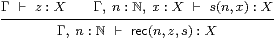
The elimination rule,
|
for which the η-rule is rec(n,0,+1)=n and the β-rules are
| rec(0,z,s) = z and rec(n+1,z,s) = s(n,rec(n,z,s)), |
defines primitive recursion at type X. We sometimes specify the type when it is necessary to restrict its generality, because some logical investigations become too difficult for arbitrary types. In symbolic logic, the defining expressions z and s are naturally understood to allow parameters, which it is the role of the context Γ to manage (§2.2).
Bill Lawvere captured these ideas categorically by observing that (ℕ,0,+1) is the free algebra for the endofunctor 1+(−); then the universal property compares it with another algebra (X,z,s). However, as with ∨ and ∃ (§5), this does not make allowance for parameters. One way to handle them is by using recursion at type XΓ, if we are working in a cartesian closed category, but our category S does not have general exponentials like this, so we shall keep the explicit parameters.
9.5.
Many familiar things can be defined by recursion on ℕ,
not least its arithmetic, but we just note those that we
shall need later in this paper.
In particular,
we may define a map cmp :ℕ×ℕ→ℕ using the equations
|
whilst φ(0)=⊥ and φ(n+1)=⊤ give one φ:ℕ→Σ. From these we derive the six relations =, ≠, <, >, ≤ and ≥ and their usual properties as terms of type Σ on ℕ, which is therefore both discrete and Hausdorff.
Notice that we distinguish the symbol ≤ for the arithmetical order from the logical order ⊑ that is defined on ΣX (§8.2). Then ≤ is imposed structure, because functions ℕ→ℕ do not have to preserve it, whereas ⇒, ⊑ and ⊑ are intrinsic, in that every morphism necessarily preserves them.
Hence, for each numeral n, the object n≡{m:ℕ ∣ m< n} may be defined as a subspace of ℕ that is both open and closed. It is also both overt and compact, with quantifiers that are definable from ∨ and ∧ by primitive recursion.
9.6.
There are tricks for encoding pairs and lists as integers,
but they are computationally expensive,
whilst logic and functional programmers have long known a better way
of doing things.
A simple modification of the definition of ℕ yields
a very useful and general data structure, T, of binary trees.
Instead of the unary successor operation for ℕ,
T has pairing, which is written [ a | b ],
whilst the projections are called car and cdr
in memory of some ancient hardware [McC78].
This is also of theoretical utility, because List (T)≅T,
where
| [a, b, c, …, z] ≡ [ a | [ b | [ c | [ … | [ z | 0 ]… ] ] ] ]. |
9.7.
Combining ℕ or T with the structure of a pretopos
gives a very expressive setting, in which we may do anything we like
of a combinatorial nature, i.e. definable using explicit enumerations.
In particular, the quotient of a finite object n by an equivalence relation is finitely generated but not necessarily finitely enumerated, i.e. it can be listed, but possibly with repetitions [Tay99, §6.5]. This weaker notion of finiteness is due to Kazimierz Kuratowski [Kur20]. It is more relevant to logic, because we may regard the free semilattice on a set as its collection of Kuratowski-finite subsets [Mik76, Appx 2], so we write K(N) for what is elsewhere called the finite powerset.
These are the properties that are taught to first year mathematics and computer science undergraduates as naïve set theory or discrete mathematics.
In category theory, an arithmetic universe is a pretopos in which any object N generates a free monoid List (N), from which we may derive K(N) and other free algebras. This notion was introduced by André Joyal in 1973, as a way of formulating Gödel’s incompleteness theorem [Göd31] in a categorical way, but unfortunately he has never published his results. Maria-Emilia Maietti has given a symbolic calculus for arithmetic universes in the style of Martin-Löf [Mai03, Mai05]. One symptom of the paucity of literature on this important topic is that some disagreement remains about the precise details of the definition, in contrast to the more rigorous attention that was given to elementary toposes (§§3.2,5.3).
9.8.
It is all very well constructing terms by recursion, but we also want
to prove properties of them by induction.
Since recursion may be used within terms, and not just on
the outside, induction does not follow directly from the rules above,
and is treated separately in symbolic logic:

|
Notice that, in order to prove some equation f n=g n:X by induction, we need to be able to state it as an induction hypothesis [Section E 2].
Categorically, induction can be treated as a special case of recursion, but only when we have the additional structure of the equaliser type:
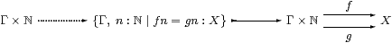
As is common with universal properties, we use them twice: once to obtain the dotted map, and again to say that the composite Γ×ℕ→Γ×ℕ has to be the identity, which we obtain symbolically from the η-rule. It follows that the inclusion into Γ×ℕ is the whole thing.
9.9. Notice that these equalisers or equational hypotheses have arisen
for logical reasons,
so I believe that we probably ought to understand them proof-theoretically
(§12).
For the time being, however,
we may give them a meaning amongst either Bourbaki spaces or locales,
in either of which we have
9.10.
The abstract theory needs to reproduce this situation.
Plainly ℕ should be a “set” in the sense of §9.2,
so we must also say that it admits existential quantification.
Besides the axioms in §§6.1 & 8.1,
we therefore require
In the symbolic language, we distinguish between types (corresponding to objects X∈S) and contexts (Γ∈L). Any type X has a topology ΣX, whilst a context Γ may include equational hypotheses, so this extension subsumes the one that we made in §8.4.
The existential quantifier ∃ℕ breaks the open–closed duality in topology, since we do not equip ℕ with a universal quantifier too. Topologically, this is because ℕ is not compact [C 7.11], whilst computationally it is not possible to observe an infinite conjunction in the way that it is a disjunction.
9.11.
Whilst ℕ exposes one flaw in the monadic framework,
in another way it shows its conceptual strength.
We call a predicate Γ⊢φ:Σℕ a description
if it ought to be “uniquely satisfied” in the sense that
| Γ ⊢ ⊤ ⇔ ∃ n.φ n and Γ, n,m:ℕ ⊢ φ n∧φ m ⇒ n=m:ℕ. |
From sobriety of ℕ (§6.3) we deduce that φ actually has a witness (definition by description), namely
| the n.φ n ≡ focusℕ(λψ.∃ m.φ m∧ψ m). |
It is easy to show that P≡λψ.∃ m.φ m∧ψ m satisfies the lattice-theoretic characterisation of primality, but use of that depends on Scott continuity (§11.6). Deducing the λ-calculus definition from primitive recursion is a little trickier [Proposition A 10.8].
Conversely, any prime P:Σ2ℕ gives a description (easily [Proposition A 10.4]. by
| φ n ≡ P(λ m.m=n). |
The defining conditions for a description and its operator, “the”, provide the introduction rule for another symbolic calculus. The elimination rule says that
| ψ(the n.φ n) ⇔ ∃ n.φ n∧ψ n, |
the β-rules justify the name “the n.φ n”,
| ⊤ ⇔ φ(the n.φ n) and φ m ⇒ m=ℕthe n.φ n, |
and the η-rule says that, for any n:ℕ, the predicate φ m≡(n=ℕm) is a description, with n=the m.φ m. Like focus, the description operator can be eliminated everywhere except on the outside of the term.
A description with parameters are is called a functional relation, and the corresponding function assigns witnesses for each value of the parameters.
Definition by description is easy to overlook as a principle of reasoning in mathematics. It was first formulated correctly by Giuseppe Peano [Pea97, §22], including the elimination theorem and the need to prove the properties of φ before introducing the n.φ n. Numerous other accounts, most notably [RW13, *14], have failed to do this. It is nevertheless much more familiar than the abstract notion of sobriety in the monadic framework, so we have another example in which different axioms are appropriate in accounts of foundations and applications (cf. §3.8).
9.12.
The notion of general recursion weakens that of
definition by description into a form that is more akin to computation.
It involves a search or minimalisation operator µ
such that, for any partial map f:ℕ⇀2,
| µ(f)=n iff f(n)=1 but ∀ m< n.f(m)=0. |
If f is total and ∃ n.(f n=1) then φ≡λ n.(f n=1)∧∀ m< n.(f m=0) is a description, for which µ(f)=the n.φ n. However, we can use Rosolini’s treatment of partial functions (cf. §7.3), together with the construction of ℕ⊥ in §8.11, to define µ(f) for all f:ℕ⇀2.
First we need the fact that 2⊥ is given by the closed subspace of Σ×Σ co-classified by λστ.σ∧τ, and (2⊥)ℕ by that of Σℕ×Σℕ co-classified by λφψ.∃ n.φ n∧ψ n.
The predicate θ n≡φ(n)∧∀ m< n.ψ m satisfies the uniqueness requirement for a description, when we restrict (φ,ψ) to the closed subspace (2⊥)ℕ⊂Σℕ×Σℕ. Then, on the open subspace P⊂(2⊥)ℕ classified by ∃ n.θ n, i.e. the uniqueness condition, θ is a description, so defines a total map P→ℕ and a partial one (2⊥)ℕ⇀ℕ. The corresponding total map µ:(2⊥)ℕ→ ℕ⊥ is the required minimalisation operator.
9.13.
Given that the entire discipline of denotational semantics of
programming languages is based on Scott continuity, it may come as a
surprise that we can interpret general recursion without using it.
This is because the (old-fashioned) search operator µ is only suitable
for direct coding using base types such as ℕ or T.
For terms and parameters of these types, Scott continuity is a theorem, essentially the one of Henry Rice and Norman Shapiro [Ric56]. For any class U of programs that is recursive enumerable using tests on their coding and pointwise values, a partial function is representable by a member of U iff it contains some function with finite support that is also representable.
Looking at this type-theoretically, Scott continuity is provable for any expression with no free variables of type higher than Σℕ. This is valid in practice for computation, because a program cannot proceed if there are any free variables (i.e. undefined values or sub-routines) at all. On the other hand, we use Scott continuity in the theory, not just to allow free variables, but because of the powerful conceptual analogy with general topology . ASD tightens this analogy by reformulating topology to fit Scott’s theory of computation exactly.
We began this section by saying that overt discrete objects play the role of sets, but we have actually only used subquotients of ℕ. We need a further assumption in order to be able to work with abstract overt discrete spaces, i.e. general types for which ∃ and = can be defined. Assuming Scott continuity, all overt discrete objects are subquotients of ℕ, and form an arithmetic universe (§11.7).