


We now sketch the technical background to our general method of developing foundations for mathematics.
2.1.
Gerhard Gentzen, the father of proof theory, set out the way in which
we reason with the logical connectives (∧, ∨, ⇒)
and quantifiers (∀ and ∃) [Gen35].
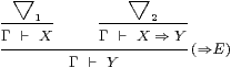
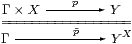
Consider, for example, how we use and prove implications (X⇒ Y). If we know both X and X⇒ Y then we also know Y; this is traditionally called modus ponens. More generally, we may have proofs ▽1 and ▽2 of X and X⇒ Y respectively, from a set Γ of assumptions. Putting these together gives a proof of Y, as illustrated on the left:
|
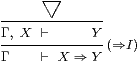
Conversely, how can we prove the implication X⇒ Y? By definition, it is by giving a proof ▽ of Y that may assume X, as on the right. We need to maintain a list Γ of such assumptions in order to keep track of the extra ones that we add and discharge in proofs of implications; this list Γ is called the context.
These two patterns are called the elimination and introduction rules for ⇒ respectively (hence the labels ⇒E and ⇒I), because of the disappearance or appearance of this symbol in the conclusion. There are similar rules for the other connectives and quantifiers.
2.2.
Under Haskell Curry’s analogy between propositions and types
[How80, Sel02],
type connectives (×, +, →) and quantifiers (Π and Σ)
were later expressed in a similar way.
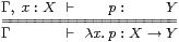
But now, in place of the bald assertion that X⇒ Y,
we now have a function X→ Y that takes values of one type
to those of the other.
This function needs a name.
Bertrand Russell [RW13, *20]
originally called it x(φ x), but the hat evolved into a lambda:
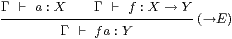
|
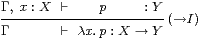
Since types come with terms, these too need rules for their manipulation. The beta rule arises from first introducing and then eliminating the symbol, and the eta rule from the converse,
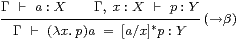
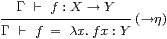
|
where [a/x]*p indicates substitution (§2.7). Now the context Γ must include both assumptions and typed variables or parameters.
2.3.
If we have such a system of rules for the connectives that we use —
instead of encoding them in a much more general and powerful
all-encompassing foundational monolith —
then we have some chance of computing in our system.
Of course, mathematicians always did that, before logicians came along:
the difference is that the system is now much bigger (§1.4),
and so requires a more formal relationship amongst its parts,
and amongst the specialists in very diverse disciplines (§3.6).
In the simply typed λ-calculus, for example, we merely have to keep applying the β-rule, and then we are guaranteed to get to the normal form ... eventually. In order to prove termination of this process we use induction on the complexity of the types that are involved. For uniqueness, we need to know that, whenever we have a choice of redexes (reducible expressions), the two results can be brought back together by further reductions [CR36]. Both of these results depend in delicate ways on the formulation of the system.
Whilst it may be rather naïve to rely on this “guarantee” in practice, we can profitably hand the formal system over to the experts in manipulating symbols. They do not need to understand their original meaning, but may use their own experience of similar systems to make the computation more efficient. Even so, it is the mathematical system — not the way in which some machine happens to work — that determines the fundamental rules. This has been done very successfully in functional programming, which is now almost as fast as machine-oriented approaches [Hud89, HHPJW07].
There is, in fact, much profit to be made from collaborating with computational specialists only via a formal language. They may be able to transform it into something entirely different, that works qualitatively faster than the methods that the mathematician originally had in mind. One example of this that is indirectly related to the ideas in this paper (§6.4) is the continuation-passing method of compiling programs, because of its similarity to the way in which microprocessors handle sub-routines [App92].
Another example arises in the solution of equations involving real numbers. Interval-halving methods are often used to prove theorems in constructive analysis (Section J 1), but if we were to compute with them verbatim we would only get one new bit per iteration. Newton’s algorithm, by contrast, doubles the number of bits each time. But the verbatim reading is a mis-communication — we only halve the interval for the purpose of explanation. A practical implementation may choose the division in some better place, based on other information from the problem. Indeed, this what is done in logic programming with constraints [Cle87]. Putting the ideas together, we can turn one algorithm into the other [Bau08][K].
Altogether, we can think mathematically in one way, but obtain computational results in another.
2.4.
Bill Lawvere [Law69] recognised the situation
in type theory (§2.2)
as a special case of that studied by categorists.
We say that the functors F :S→A and U :A→S
between categories
A and S are adjoint (F ⊣ U )
if there is a bijection (called transposition)
between morphisms
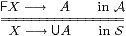
|
that is natural in X and A, which means that it respects pre- and post- composition with morphisms in the two categories. The transposes of the identities on F X and U A are called the unit and counit of the adjunction, respectively,
| ηX:X→ U (F X) and εA:F (U A)→ A, |
and these satisfy equations known as the triangle laws:
| U εA·ηU A = idU A and εF X· F ηX = idF X. |
The use of the letter η for different things in category theory and type theory is most unfortunate, but it is a historical accident that is very well established in both subjects.
2.5.
For example, the correspondence
 or
or
|
is bijective on the left by the symbolic rules (§2.2), and on the right as the adjunction (−)× X⊣ (−)X. However, purely categorical textbooks cover many pages with diagrams expressing arguments that could be written much more briefly by adopting the notation λ x.p instead ∼ p (cf. §6.1).
This analogy can be followed systematically through all of the logical connectives:
The reason why some of the connectives (⇒, ∧, →, ×) work one way round and the others (∨, ∃, +) differently is that they are respectively right and left adjoints to something that is simpler. This is described more fully in [Tay99, §7.2].
2.6.
In order to formalise this relationship between adjunctions and
systems of introduction, elimination, β- and η-rules,
we need a fluent translation between diagrammatic and
symbolic languages.
In fact, we just require a way of turning a type theory that has all of
the structural rules
(called identity, cut, weakening, contraction and exchange
in proof theory) into a category with finite products.
Then we can when this category obeys other universal
properties, reading the corresponding symbolic rules off from them.
The following method also works for dependent types, i.e. possibly containing parameters, but we shall avoid them in this paper. There are, conversely, ways of defining a language from a pre-existing category [Tay99, §7.6], but these are more complicated and will not be needed here. Systems such as linear logic that do not obey all of the structural rules correspond to different categorical structures. These structures might, for example, be tensor products (⊗), which categorists understood long before they did predicate logic [ML63]. It is therefore often the syntax that requires the most innovation, for example using Jean-Yves Girard’s proof nets [Gir87].
A type theory L of the kind that we shall consider has recursive rules to define
2.7.
We have already used the substitution operation [a/x]*c,
which must be defined carefully in order to avoid variable capture
by λ-abstraction.
Another operation
(called x* c in [Tay99, §1.1]
but not given a name elsewhere) weakens c
by pretending that it involves the actually absent variable x.
These satisfy the extended substitution lemma,
| [a/x]*[b/y]*c = [[a/x]*b/y]*[a/x]*c [x/y]* |
| *[y/x]* |
| *c = c |
| [a/x]* |
| *c = c [a/x]* |
| *c = |
| *[a/x]*c |
| * |
| *c = |
| * |
| *c |
where x≢y, x,y∉FV(a) and y∉FV(b).
2.8.
Like so many other operations in mathematics,
substitution is defined by its action on other objects.
So, when we abstract the operation from its action,
it has an associative law of composition,
which brings it into the realm of category theory.
The objects of the category are, abstractly, the contexts Γ of the type theory. More concretely, Γ is represented by the set of terms that are definable using free variables chosen from Γ. The substitution and weakening operations define morphisms
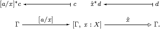
It is convenient to draw the arrows in such a way that substitution looks like inverse image, which is why we write it with a star. We also draw weakening with a special arrowhead and call it a display map. The five equations of the extended substitution lemma say that certain diagrams formed from these arrows commute, i.e. segments of paths of arrows that match one pattern may be replaced by another. For example, the composite of the two arrows above is the identity.
Altogether, we have defined, not the category itself, but an elementary sketch . That is, whilst we have spelt out all of the objects, we have only given a generating set of arrows. The category CnL× itself consists of all paths formed from these arrows, subject to the equations of the given symbolic theory L and those of the extended substitution lemma. There is a normalisation theorem that says that any morphism Γ→Δ is essentially an assignment to each variable in Δ of a term of the same type, but formed using variables from the context Γ. In keeping with the traditional names of categories (“of objects X and morphisms Y”), We therefore call this the category of contexts and substitutions. The details of this construction are given in [Tay99]: see §4.3 for the simply typed case and Chapter VIII for its generalisation to dependent types.
The category CnL× has the universal property that interpretations of the theory L in another category T correspond bijectively (up to unique isomorphism) to functors CnL×→T that preserve the relevant structure. This means that it is the classifying category for models of this structure.
Type theories are presented in a recursive fashion, whilst categories have associative composition, but anyone who has written any functional programs knows that associativity and recursive definitions do not readily mix. Andrew Pitts defined the classifying category in this way in [Pit01, §6]; it was the complexity of even showing that the identity is well defined as a morphism in this approach that led me to the construction via a sketch. It demarcates the things that are naturally described in a recursive and symbolic way from those that are best done associatively and diagrammatically.
2.9.
Many of the comparisons and contrasts between the diagrammatic and
symbolic presentations are illustrated by Lawvere’s
notion of hyperdoctrine [Law69],
which we mention as a methodological example rather than for technical reasons.
A hyperdoctrine represents the quantifiers Π and Σ
as the right and left adjoints (cf. §2.5)
to the substitution functors
f*:A[Y]→A[X] that are defined by a map f:X→ Y.
However, induced and restricted modules along a ring homomorphism
also provide adjunctions like these.
The difference is that, in symbolic logic, we may substitute
for parameters within the scope of the quantifiers.
This is not part of the correspondence in §2.5,
so category theory must express it by another axiom,
known as the Beck–Chevalley condition,
which does not hold for general ring homomorphisms.
Another property that is peculiar to the existential quantifier
is the equation σ∧∃ x.φ x⇔∃ x.σ∧φ x,
which Lawvere called the Frobenius law
on the basis of analogies with linear algebra.
So category theory is
On the other hand, it is
2.10.
Another criticism of hyperdoctrines is that,
in requiring this structure for all maps f:X→ Y,
they have a hidden bias towards set theory.
The same remark applies to type theories that
allow quantification over types with arbitrary parameters.
In order to apply Lawvere’s ideas to topology or domain theory
(for example, to model second-order quantification over type variables),
we must restrict the subclass of maps that admit quantification.
It is more accurate to say that quantification
is adjoint to weakening [Tay99, Ch. IX].
In this paper, set theory will be important, neither as the standard or a competing logical theory, but as an analogous mathematical one, providing another example of Stone duality (§4.5). We aim to study topology, which is about continuous things, so by “set theory” here we shall mean any treatment of discrete objects, which may be in an elementary topos, using type theory or in some axiomatisation of the ∈-relation.
The key difference that will emerge is that in the logic of discrete things we may use quantifiers ranging over any object, whilst in topology only some spaces may play this role. An object X that may serve as the range of a universal quantifier is called compact. More generally, a map that admits parametric universal quantification à la Lawvere is called proper, and we think of the map as a continuous family of compact spaces. Similarly, a map with existential quantification is open, but we need to introduce a new word, overt, for the corresponding objects.
2.11.
Nevertheless, Lawvere’s insight is the key to our method,
when we turn it around.
Having seen many systems of rules and adjunctions for different logical
connectives, we may recognise the general pattern and apply it to
mathematics.
Many theorems in mathematics (our client’s brief) may be formulated as adjunctions, to which we apply Lawvere’s correspondence in reverse: we invent new symbols whose introduction, elimination, abstraction, beta and eta rules exactly capture the adjunctions. We shall do this in §6.3 for sobriety, in §§6.6f for Σ-split subspaces, in §9.11 for definition by description, in §10.6 for underlying sets, in §11.11 for Dedekind completeness and in §12.3 for more general subspaces.
2.12.
The new symbols are not meant to be merely abbreviations for
common lemmas about the old structure, but to stand on their own feet
as principles of reasoning in the new one.
As with complex numbers (§1.3), we want to be able to compute
with them without having to worry about what they mean (§2.3).
This means that we need to ensure that they are accompanied by
a complete set of rules of inference
and show that they are conservative over simpler systems.
One good indicator of sufficiency is being able to prove a normalisation theorem. Typically, this says that say that any term that makes arbitrary use of the introduction and elimination rules is provably equivalent to one that uses
The equivalence between the categorical and symbolic constructions, and conservativity, are deduced from theorems of this kind, and will be a key step in the general method that we now propose.